Research Article, Geoinfor Geostat An Overview Vol: 5 Issue: 2

Slope-Independent Landscape Roughness Attribute Provided by Measurement of Local Contour Line Density

Veronica Ochoa-Tejeda^1* and Jean-François Parrot²

¹SERTIT (Service Régional de Traitement d’Images et de Télédétection), Université de Strasbourg, Boulevard Sébastien Brant, 67412 Illkirch, France

²Instituto de Geografia, Universidad Nacional Autonoma de Mexico, Circuito Exterior, Ciudad Universitaria, Coyoacan, 04510, Mexico

Corresponding author : Veronica Ochoa-Tejeda
SERTIT, Université de Strasbourg, Boulevard Sébastien Brant, 67412 Illkirch, France
Tel: + 33 (0) 786011897
E-mail: veronikot11@yahoo.fr, parrot@igg.unam.mx, jfparrot@hotmail.com

Received: February 02, 2017 Accepted: February 16, 2017 Published: February 21, 2017

Citation: Ochoa-Tejeda V, Parrot J (2017) Slope-Independent Landscape Roughness Attribute Provided by Measurement of Local Contour Line Density. Geoinfor Geostat: An Overview 5:3. doi: 10.4172/2327-4581.1000159

Abstract

Keywords: DEM’s surface roughness; Contour line density; Slope independent roughness parameter; Geomorphic features; Sierra Norte de Puebla

Introduction

Raster digital elevation models (DEMs) are nowadays widely used, since advances in computing technology and storage have increased strongly in recent years. The horizontal and vertical resolutions allow accurate calculation of parameters extracted from a DEM surface. Digital terrain analysis [1] allows definition of primary attributes calculated directly from the DEM surface (i.e. slope, aspect, plan and profile curvature) and secondary attributes whose calculation requires external information and that are more devoted to estimating the role of topography in the distribution of soil water or in the susceptibility of landscapes to erosion, for instance. Most of the primary attributes are computed directly with a finite-difference scheme or by fitting an interpolation function Z=f (x,y) to the DEM in order to calculate the derivatives of this function [2-5]. These attributes provide numerous geomorphologic indicators concerning the region under study [6]. They are used to describe the morphometry, catchment position, stream channels and other factors and to compute topographic attributes [7-12]. Several recent pedologic and geomorphologic applications are based on features automatically extracted from DEMs. The publications concerning this topic were surveyed by Pike [13]. Various softwares described in Gallant and Wilson [14] has been developed for the parametric study of gridded DEM surfaces.

Geomorphometric features such as the surface roughness of a DEM provide information about regional geomorphology, and many roughness parameters have been proposed. For instance, the fractal dimension can be considered as an indicator for terrain surface roughness in DEMs [15-18]. Other authors used parameters of curvature to analyse the surface locally [19-22]. Curvature attributes are useful for measuring flow convergence and divergence [23] and for defining geomorphic units [8], and they can be calculated by using a bi-quadratic surface to classify the types of surface [20,22,24].

Moreover, Teng and Tay [25] suggested defining a simple and easily computed surface roughness index RI based on the differences of heights between neighbouring pixels within a window. Dinesh [26] proposed a procedure to compute a scale-independent surface roughness parameter from DEMs and extended this method to compute the surface roughness of individual mountain objects extracted from DEMs by means of mathematical morphology [27]. With a similar purpose, Hebeler and Purves [28] assumed that topographic indices calculated by the software GLOBE [29] such as Altitude Roughness (standard deviation of altitude in a 3 × 3 neighbourhood) and the Slope Roughness (standard deviation of slope in a 3×3 neighbourhood) are sufficient to study the influence of elevation uncertainty on derivation of these indices. Gallay et al. [30] analysed the elevation error of high-resolution DEMs by using the roughness index defined by Fisher and Tate [31]. In this case, the area ratio roughness would correspond to the ratio of real surface area to the area of its orthogonal projection [32,33].

However, for most of these treatments, the expression of the surface roughness is too closely related to the slope. Therefore, we tried to develop a surface roughness measurement that is independent of the slope values. The calculation of this new attribute is based on the measurement of the total length of a given number of contour lines extracted inside a moving window of nn pixels. As the number of extracted contour lines remains unchanged, the range of the hypsometric intervals varies according to the slope value, i.e. the total length of the contour lines depends only on the design they draw according to the roughness of the moving window surface.

To illustrate the geomorphologic information provided by this new parameter, the treatment has been applied to the region of La Soledad, Sierra Norte de Puebla, Central Mexico, where numerous mass movements occurred in 1999 and 2005. A close relationship occurs between the position of the landslide starting points and the smooth zones supplied by the new roughness attribute called the Slope-Independent Roughness Parameter (SIRP).

Ochoa-Tejeda [34] studied the distribution of all the landslides that occurred in this region in 1999 and measured the relative influence of various factors related to mass movements: geological units, geomorphologic parameters and primary attributes such as slope, aspect, convexity, energy of the relief, drainage density and vegetation density [35] as well as the local 3D fractal dimension [18]. Another approach related the morphology of the landslide traces with the nature of the material remobilized during the event [36].

In 1999, Tropical Depression N° 11 coming from the Gulf of Mexico triggered more than 3000 mass movements related to the torrential and sudden rainfalls of 4-5 October [37]. Data from the Mexican National Meteorological Service indicate that the amount of rain during the first days of October considerably exceeded the monthly and annual average values. For instance, in Zacapoaxtla, the accumulated precipitation during the 4 days of 3-6 October was 844 mm, i.e. 60% of the annual average of 1421.2 mm.

In 2005, from 1 to 4 October, hurricane Stan produced intense rains in the northern region of Puebla with a peak of 273 mm during 24 h. In addition, Tropical Depression N° 40 interacted with the hurricane from 4 to 6 October causing rains of up to 305 mm in 24 h. This phenomenon was responsible for severe soil saturation and water flows [38]. The effect of rain depends basically on the intensity, duration and distribution of the storm. Manzini and Rabufetti indicate that when the superficial formations are constituted by clastic and colluvial soils, the precipitation threshold that produces shallow landslides is related to the inclination of the slope, the infiltration and the loss of apparent cohesion.

The results obtained in this test region show that the SIRP clearly emphasizes the different roughness zones according to the size of the moving window.

Material and Methods

Derivation of the roughness attribute

To calculate the contour-line density inside a moving window of size n×n, it is first necessary to take out, one by one, each contour line extracted from the DEM according to the hypsometric interval retained by the user. At each step, all the pixels that are lower than or equal to a given elevation are reported in a temporary image. Then a treatment in this matrix ensures the extraction of the contour lines from the corresponding zone. A plain procedure consists of considering that a pixel defines a contour line (Figure 1A) when at least one of the cardinal neighbouring pixels does not belong to its corresponding extracted zone (Figure 1A). When necessary, the remaining corners are eliminated in order to obtain an 8-vicinity curve, i.e. a curve formed by segments of 1 to n pixels linked only by their corners.

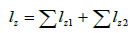
The length of this contour line is calculated as follows. One can consider, within the pixel surface, the value of one-half of the straight line that links the pixel centre and the centre of the neighbouring pixels. In this case (Figure 2), and according to the configuration encountered in a test 3×3 pixel window, the two lines values d_z1 and d_z2 encountered within the pixel surface are respectively equal to ½ and to of the cell size (P_s). The value d_z1 is applied to the cardinal neighbours and the value d_z2 is used when the pixels are diagonal neighbours.

Taking into account the cell size P_s, the algorithm calculates the lengths l_z1 and l_z2 encountered in the 3 × 3 pixel window. The computation is done in this way:

(1)

Where l_z1 = d_z1× P_s and l_z2 = d_z2×P_s

When strong escarpments are present, it is not rare for a pixel to register more than one contour line, since for a low hypsometric interval value successive contour lines may pass through the same point. The total length L_z corresponds to the sum of all the local values L_z obtained. According to the raw order, this calculation is done for each pixel of each extracted contour line in order to avoid any coalescence between contour lines such as they appear in Figure 1. The value obtained is reported in a float matrix and eventually summed to a pre-existing value.

In the example of the three contour lines reported in Figure 1, L_z is 29.796. For instance, if the value of the pixel side P_s is 25 m, the total length for the three contour lines encountered in the moving window is 744.9 m.

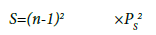
The size of the moving window side n corresponds to an owe value (i.e. 11 × 11 pixels in this example). The surface S where the three curves are emplaced (Figure 1) is equal to n-1×n-1, (here 10 × 10 pixels), because when a pixel is on the window border there is no information about the pixels neighbouring emplaced throughout this window. In this case, the surface S is equal to:

(2)

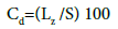
For the pixel side P_s formerly proposed, S corresponds to 62 500 m² in such a way that the Density of the Contour Lines in the moving window is equal to:

(3)

For example, C_d is 1.146 in the case of the contour lines reported in the Figure 1. At the end of the treatment, normalization (0, 100) can be operated in order to obtain the C_d percentage reported in an image of the Contour Line Density (CLD).

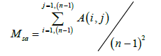
In order to compare the results obtained using the calculation of the contour line length inside a moving window on a training zone with the slope values, the mean slope angle M_sa has been calculated in a moving window that has the same size:

(4)

where n is the number of the pixels encountered in the moving window and A the angular value of each pixel in this window.

Slope-independent approach

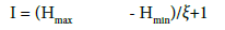
As the CLD is related mainly to the terrain slope, another approach has been developed. The calculation of the “Slope-Independent Roughness Parameter” or SIRP consists of applying the former algorithm inside a n × n moving window taking into account the local difference observed between the upper and lower altitudes inside the moving window. Although this calculation is computationally intensive, its results are more consistent with the “roughness” notion. The upper and lower hypsometric values (H_max and H_min) observed inside the moving window allow calculation of the local hypsometric interval H used to extract the contour lines dividing the difference between H_max and H_min by ξ+1, where ξ corresponds to the number of required contour lines.

(5)

The value of I allows the same number of contour lines to be drawn in each successive moving window.

Following the procedure described above (Figure 1) all the pixels that are lower than or equal to the succeeding altitude levels are reported in a temporary n×n matrix; the pixels describing the perimeter of the consecutive slices thus obtained correspond to a contour line. The length of the line crossing each pixel belonging to the contour line is calculated according to the formula (1) and the total length L_z of this contour line corresponds to the sum of all the local values l_z obtained. As previously, the surface where the three curves are emplaced is equal to n-1 × n-1, and the SIRP is calculated according to the equation (3).

Case Study

Validation and control of the results used a DEM of one region from the Sierra Norte de Puebla (Central Mexico) that has a surface area of ~135 km². This region was affected by torrential rainfalls in October 1999, producing numerous landslides and flooding [39-41]. In the whole region, about 3000 mass movements occurred, consisting of rock and soil slides and slips, debris flows and avalanches. Capra et al. [41] identified two types of mass movements in the Teziutlan volcanic area: a) small detrital fans especially in the ignimbrite formations; and b) soil slide/debris flow in the volcanic sequence. In the region of Zapotitlán de Méndez [42] rotational landslides affected folded shales. The study region (19° 53’-20° 00’ N and 97° 24’-97° 25’ W) lies between the Sierra Madre Oriental geological province and the northern border of the oriental part of the Trans- Mexican Volcanic Belt (Figure 3). The main geological units [43] are the Paleozoic formations mainly formed by mylonitized schist, discordant Jurassic formations (sandstones and marls in the lower sequences and limestone in the Upper Jurassic), Cretaceous limestone of Neocomian age and Tertiary and Quaternary volcanic flows (Pliocene andesites and Quaternary ignimbrites). With the exception of these volcanic formations, numerous necks, dykes and sills of rhyolitic composition intrude throughout the stratigraphic sequence.

The DEM results from an interpolation [44,45] taking into account the contour lines digitized from the INEGI topographic map of the region (1/50 000). The resulting DEM has 2374 rows and 2270 columns (Figure 4). The pixel size is 5 m and the elevation is in decimetres. Even if this DEM presents some artefacts inherent to this type of interpolation that over-estimates the number of pixels describing the contour lines, a light smoothing blurs these defaults because the hypsometric scale is in centimetres and the result is good enough to calculate in an accurate way the indices described above.

Results and Discussion

General contour line density

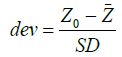
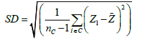
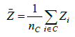
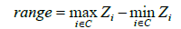
The result does not present the artifacts observed in the case of different primary attributes such as, for example see [1] the “deviation from mean elevation” (formula 5, 6 and 7) that is supposed to emphasize the local surface roughness or the “elevation range” (formula 8) that produces visible overlapping circular regions (Figure 5). These attributes are respectively calculated as follows where the set of cells included in the circle about the point being considered is denoted by C, and the number of cells in the circle is n_C.

(6)

Where the Standard deviation SD and the mean �?�?Z (Z corresponds to the altitude inside the circle) are calculated as:

(7)

(8)

(9)

But even if the resulting image underlines some geological features, the CLD remains too closely related to the slope values. In fact, on the scatter plot CLD versus Slope (Figure 6), the normal trend has a high correlation coefficient of 0.7319.

Slope-independent roughness parameter

The calculation that takes into account the local hypsometry inside the moving window offers a completely different result. As the number of contour lines extracted inside the moving window depends on the hypsometric difference between the upper and lower altitude, and remains always equal to a given number (3 for example), the contour line complexity is related only to the roughness of the DEM surface observed inside the moving window. For instance, a flat zone will have the same total length L_z and the same contour line density regardless of the slope value.

Figure 7 illustrates the result obtained using 11×11 moving window size. The scatter plot “Slope Independent Roughness Parameter [SIRP]” versus Slope (Figure 8) clearly shows that the measurement is not related to slope values. The corresponding coefficient of correlation is in this case –0.043.

Discussion

The SIRP is a new morphometric parameter directly issued from the DEM surface. As shown above, this primary attribute is not related to the corresponding local slope and can be used to provide information about the different types of landslides observed in the study region.

In Figure 9, the grey tone (from light to dark) shows the slope value (11°-20°, 21°-30°, 31°-40°, >41°) inside the segment 14-25 of the SIRP histogram (Figure 10). Lower values of the SIRP histogram are essentially associated with the La Soledad Lake.

A close relationship exists between the low values of the SIRP and the landslides distribution. More than 80% of the 1999 landslides and 75% of the 2005 landslides are in smooth zones (Figure 10). Hence, roughness might somehow represent an obstacle to the triggering of shallow landslides. The landslides related to very rough zones represent 5.75% in 1999 and 5.20% in 2005. They mainly affected the rhyolites in 1999 and the Upper Jurassic cliffs in 2005, producing rock avalanches and debris flows.

Within the smooth zones, the distribution of landslide starting points in relation to slope values (Figure 10) was similar between 1999 and 2005 except for the lowest slope vales, where the percentage was greater for 2005. This slight difference may be related to the nature of the tropical depressions that affected the mountainous zone of the state of Puebla, mainly in its northern region, in October 1999 and October 2005, as well as the different types of material involved.

According to these observations, it seems that soil saturation in October 2005 was responsible for the development of mass movements affecting essentially superficial formations. This observation is corroborated by the landslide distribution according to the geological units where the increased percentage in 2005 concerns the Quaternary ignimbrites and the superficial formations related to the Middle Jurassic and the metamorphic formations.

Conclusion

The aim was to define a roughness parameter derived from the gridded surface of the DEM in order to obtain morphometric information concerning geomorphologic studies. The Slope- Independent Roughness Parameter is a new primary attribute that is not closely related to the slope and thus represents a powerful indicator of the DEM surface roughness.

Its application to the distribution of mass movements that occurred in the Sierra Norte de Puebla (Mexico) during October 1999 and October 2005 shows that the superficial and shallow landslides are closely related to the smooth zones. They are essentially debris flows that are generated when hillside colluvium or landslide material becomes rapidly saturated, as well as mudflows, creeps and eventually lateral spreads. Falls involving rocks and boulders detached from steep slopes or cliffs, and rock avalanches occurred in zones of high roughness because the mobilization of the material is mainly related to discontinuities such as fractures, joints and bedding planes. They produce coarse deposits in talus and talus breccias and sometimes colluvium easily remobilized by torrential rainfalls.

The SIRP is a useful parameter that can be used in tandem with other pertinent parameters such as slope angle, aspect or concavity in order to map the susceptibility of hillslopes to mass movements.

References

1. Wilson JP, Gallant JC (2000) Terrain Analysis. Principles and Applications. John Willey & Sons, New York.
2. Moore ID, Lewiss A, Gallant JC (1993) Terrain attributes: estimation methods and scale effects. In: Jakeman AJ, Beck MB,.McAleer MJ, Modeling Change in Environmental Systems, New York, Willey
3. Mitasova H, Hofierka J, Zlocha M, Iverson LR (1996) Modeling topographic potential for erosion and deposition using GIS. International of Geographical Information Systems 10: 611-618
4. Florinsky IV (1998) Accuracy of local topographic variables derived from digital elevation models. International Journal of Geographical Information Science. 12: 47-62
5. Florinsky IV (2012) Digital Terrain Analysis in Soil Science and Geology. Academic Press, Oxford
6. Tribe A (1991) Automated recognition of valley heads form Digital Elevation Models. J. Earth Surface and Landforms 16: 33-49
7. Jenson SK, Domingue JO (1988) Extracting topographic structures from digital elevation model data for geographic information system analysis. J. Photogram. Eng. and Remote Sens 54: 1593-1600
8. Dikau R (1989) The application of a digital relief model to landform analysis in geomorphology. In: J. Rapper (ed.): Three Dimensional Applications of Geographic Information Systems. London, Taylor & Francis.
9. Moore ID, Gallant JC, Guerra L, Kalma JD (1993a) Modeling the spatial variability of hydrological processes using GIS. In: K. Kovar & H.P. Nachtnebel (eds.), International Association of Hydrological Sciences Publication 211: 83-92.
10. Dymond JR, Derose RC, Harmsworth GR (1995) Automated mapping of land components from digital elevation data. Earth Surface Processes and Landforms. 20: 131-137
11. Giles PT (1998) Geomorphological signatures: classification of aggregated slope unit objects from digital elevation and remote sensing data. Earth Surface Processes and Landforms. 20: 581-594
12. Borrough PA, Van Gaans PFM, MacMillan RA (2000) High-resolution landform classification using fuzzy k-means. J. to Fuzzy Sets and Systems 113: 37-52
13. Pike RJ (2002) A bibliography of Terrain Modeling (Geomorphometry). The Quantitative Representation of Topography. U.S. Geological survey Open-file report: 02-465
14. Gallant JC, Wilson JP (2000) Primary topographic attributes. In: Wilson & Gallant (Ed.): Terrain Analysis. Principles and Applications, John Willey & Sons, New York
15. Clarke KC (1986) Computation of the fractal dimension of topographic surfaces using the triangular prism surface area method. Computersand Geosciences. 12(5) : 713-722
16. Huang J, Turcotte D (1990) Fractal Image Analysis: Application to the Topography of Oregon and Synthetic Images. J. Optical Society of America A 7: 1124-1130
17. Klinkenberg B, Goodchild MF (1992) The fractal proprieties of topography: a comparison of methods. Earth Surface Process and Landforms. 17(3): 217-234
18. Taud H, Parrot JF (2005) Measurement of DEM roughness using the local fractal dimension. J. Géomorphologie 4: 327-338
19. Haralick KF (1983) Ridges and valleys on Digital images. Computer Vision Graphics Image Processing. 22: 28-38
20. Peet FG, Sahota TS (1985) Surface curvature as a measure of image texture. IEEE Transaction on Pattern Analysis and Machine Intelligence 7: 734-738
21. Philipp S, Smadja M (1994) Approximation of granular textures by quadratic surfaces. J. Pattern Recognition 2: 1051-1063
22. Cocquerez JP, Philipp S (1995) Analyse d’images: filtrage et segmentation. Ed. Masson
23. Mitasova H, Hofierka J (1993) Interpolation with regularized spline with tension, II: application to terrain modeling and surface geometry analysis. J. Math. Geol 25: 657-669
24. Besl PJ, Jain RC (1986) Invariant surface characteristics for 3D-object recognition in range images. Computer Vision Graphics Image Processing 33: 33-80
25. Teng HT, Tay LT (2006) Surface Roughness Index for SAR Image and DEMs. In IEEE International Conference on Geoscience and Remote Sensing Symposium, 2006.IGARSS
26. Dinesh S (2007) Characterization of areas of pixels modified during the generation of multiscale digital elevation models. J. Applied Sci 7: 3069-3074
27. Dinesh S (2008) Computation of surface roughness of mountains extracted from digital elevation models. J. Applied Sci 8: 262-270
28. Hebeler F, Purves RS (2009) The influence of elevation uncertainty on derivation of topographic indices. J. Geomorphology 111: 4-16
29. GLOBE Task Team et al., 1999. The Global Land One-kilometer Base Elevation (GLOBE) Digital Elevation Model, Version 1.0
30. Gallay M, Lloyd C, McKinley J (2010) Using geographically weighted regression for analyzing elevation error of high-resolution DEMs. Accuracy 2010 Symposium, Leicester, UK
31. Fisher PF, Tate NJ (2006) Causes and consequences of error in Digital elevation models. Progress in Physical Geography 30: 467-489
32. Bivand RS, Pebesma EJ, Gomez-Rubio V (2008) Applied spatial data analysis with R. New York, Springer
33. Ochoa-Tejeda V, Parrot JF, Fort M, De Fraipont P (2012) Percentage of surface increasing when passing from 2D to 3D-space used as a maorphologic parameter. Application to the study and characterization of the Sierra Norte de Puebla geological formation, Mexico. 2012.IGARSS
34. Ochoa-Tejeda V (2004) Propuesta metodologica para el estudio de inestabilidad a partir de los MDT y la Percepción Remota. Master Thesis, UNAM
35. Alcantara-Ayala I, Esteban-Chavez O, Parrot JF (2006) Landsliding and deforestation: a diachronic analysis of hillslope instability distribution. J. Catena 65: 152-165
36. Ochoa-Tejeda V, Parrot JF (2007) Extracción automatizada de trazas de los deslizamientos utilizando un modelo digital de terreno e imágenes de satélite de alta resolución. Ejemplo de aplicación: La Soledad, Sierra Norte, Puebla, México. Revista Mexicana de Ciencias Geológicas 24: 354-367
37. Bitran D, Reyes C (2000) Evaluación del impacto económico de las inundaciones ocurridas en octubre de 1999 en el Estado de Puebla. In: Bitran D, Evaluación del impacto socioeconómico de los principales desastres naturales ocurridos en la República Mexicana durante 1999. Cuadernos de Investigación 50. CENAPRED
38. Eslava-Morales H (2006) Caracteristicas del Huracan “Stan” en Puebla. In Caracteristicas e impacto socioeconomico de los principales desastres ocuridos en la Republica mexicana en el año 2005, Serie Impacto socioeconomico de los desastres en Mexico, CENAPRED 7: 177-207
39. Vazquez-Conde MT, Lugo-Hubp J, Matias LG (2001) Heavy rainfall effects in Mexico during early october 1999. In: Gruntfest E, Handmer J
40. Lugo-Hubp J, Vazquez-Conde MT, Melgarejo-Palafox G, Garcia-Jimenez F, Matias- Manzini M, Rabufetti D (2001) Sensitivity of rainfall threshods triggering soil slip to soil hydraulic parameter on hillslope geometry. Internat. Conference on fast slope movements, prediction and prevention for risk mitigation, Napoli, Italy
41. Capra L, Lugo-Hubp J, Borselli L (2003a) Mass movements in tropical volcanic terrains: the case of Teziutlan (Mexico). J. Eng. Geol. 69: 359-379
42. Capra L, Lugo-Hubp J, Davila-Hernandez N (2003b) Fenómenos de remoción en masa en el poblado de Zapotitlan de Mendez, Puebla: relacion entre litología y tipo de movimiento. Revista Mexicana de Ciencias Geológicas 20: 95-106
43. Angeles-Moreno E, Sánchez-Martinez S (2002) Geología, geoquímica y geología estructural de las rocas del basamiento del macizo de Teziutlan, Estado de Puebla. Tesis, Facultad de Ingenieria, UNAM, México
44. Taud H, Parrot J-F, Alvarez R (1999) DTM generation and contour line dilation. J. Comp. and Geosci. 25: 775-783
45. Parrot JF, Ochoa Tejeda V (2016) Generación de Modelos Digitales de Terreno raster. Método de digitalización.Geografía para el Siglo XXI. 2° Ed. Serie Textos universitarios, Instituto de Geografía UNAM