Spanish
  Chinese
  Russian
  German
  French
  Japanese
  Portuguese
  Hindi
Hindi Research Article, J Biodivers Manage Forestry Vol: 6 Issue: 4
Cost-Efficiency of Alternative Forest Conservation Targets, a Case Study from Finland
Anssi Ahtikoski*, Riitta Hänninen, Jouni Siipilehto, Jari Hynynen, Juha Siitonen, Terhi Koskela and Soili Kojola
Natural Resources Institute Finland, Paavo Havas Road 3 90014 University of Oulu, Finland
*Corresponding Author : Anssi Ahtikoski
Natural Resources Institute Finland Paavo Havas Road 3 90014 University of Oulu, Finland
Tel: +358295324416
E-mail: anssi.ahtikoski@luke.fi
Received: October 04, 2017 Accepted: November 17, 2017 Published: November 25, 2017
Citation: Ahtikoski A, Hänninen R, Siipilehto J, Hynynen J, Siitonen J, et al. (2017) Cost-Efficiency of Alternative Forest Conservation Targets, a Case Study from Finland. J Biodivers Manage Forestry 6:4. doi: 10.4172/2327-4417.1000189
Abstract
Temporal contracts to protect biodiversity in forests are a recent approach which has shown to be a promising and cost-efficient procedure. With respect to cost-efficiency of temporal contracts the relevant issue is the goal of conservation: for instance, are we interested in enhancing CWD index (coarse woody debris) or increasing the amount of dead wood in forests? This study focuses on demonstrating the effect of conservation goal (either enhancing CWD index or increasing the amount of dead wood) on costefficiency by optimization. Further, we analyze whether both the length of temporal conservation (10 or 30 years) and discount rate (2% or 4%) would have an effect on optimal solutions. The data consisted of 20 measured forest sites with stand age between 60 and 160 years. Majority of the stands (80%) fulfilled the biological conservation criteria of the Finnish Forest Biodiversity Programme METSO and a few of the stands were managed commercial forests. For temporal conservation (either 10 or 30 years), stand growth and dynamics of decaying wood were forecasted with a stand simulator (Motti) by prolonging the clear-cut with 10 or 30 years. The results for the two alternative conservation periods were compared to business-as-usual, BAU, with respect to income losses. Then, for ecological responses the initial, measured stand characteristics were set for the baseline to which temporal conservation alternatives (10 or 30 years) were compared to. The results of optimization distinctively demonstrated that the conservation goal has a relevant effect on the cost-efficiency. Further, the length of the conservation period has also an important role in cost-efficiency whereas the discount rate plays only a minor role in this study context. In the optimal solutions the forest sites with distinctively above-average initial amount of dead wood and excellent growth predictions which imply lower than average income losses due to conservation shone through with respect to cost-efficiency. As a word of caution, it should be pointed out that if one merely chooses the most cost-efficient sites for conservation, there is a possibility that a desirable level of biodiversity might not be fulfilled. To test this, the study needs to be next extended to landscape level with larger data input.
Keywords: Biodiversity conservation; Boreal forests; Cost-efficiency; Income loss; Motti simulator; CWD index; Private forest owner; Optimization
Introduction
Forests support about 65% of the world’s terrestrial taxa [1]. Conserving forest biodiversity is therefore a critical task [2]. In general, the human use of forests changes and destroys the habitat for many forest-living organisms [3]. The background for this is the increased use of forests for commercial wood production, and also the forest land is increasingly allocated to other purposes. The current climate policy targets increase demand for renewable raw materials, bio products and bioenergy implying higher demand pressures for the use of wood.
Particularly in the boreal forests, intensive management for timber production has considerably decreased habitat quality [4]. Traditionally there have been two approaches to preserve biodiversity in forests: forests can be set aside as permanent reserves or the management of the production forests can be adapted to take account for biodiversity issues [5]. Recently a third approach has been applied in biodiversity conservation in forests, namely a temporal conservation [6,7]. In brief, temporal conservation refers to a voluntary contract in which landowner is required to delay forest harvests until a specific time period. In most cases the conservation contracting also results in the harvest is being delayed beyond commercially optimal rotation period [8]. In economic point of view, regardless of the approach to enhance biodiversity (permanent conservation, temporal conservation or adapted management), the key issue is the cost-efficiency of the selected action. It means that a given cost spent on the environment (here enhancing biodiversity in forest) improves environmental quality as much as possible, or stated differently, the cost for a given level of environmental quality is as low as possible [9].
There is evidence that permanent conservation might be the most expensive measure to enhance biodiversity [9,10]. However, permanence is a speculative issue in case of assessing ecological responses [11]. On the other hand permanent conservation produces, for instance, the best substrate availability for red-listed saproxylic organisms [12]. Adapted, i.e. altered, forest management includes measures such as retention of living trees at harvest, artificial creation of high stumps, prolongation of the rotation period and retention of naturally dying trees [9,12]. Results on cost-efficiency of adapted management indicate that some silvicultural measures are more cost-efficient than others [5,9,13] but also climatic conditions has a considerable impact on cost-efficiency of adaptive management [12]. Stated differently, the most cost-efficient silvicultural measure to enhance biodiversity seems to change along with the climatic conditions, which has to be taken into account when the adaptive management procedures are applied. Recent studies indicate that both short and long-term temporal contracts for biodiversity conservation may be cost-efficient to apply in privately owned land [7,11]. Further, managed stands are more cost-efficient to be assigned mainly shortterm contracts while for unmanaged (i.e., no thinnings applied) stands both short-and long-term contracts should be used [7]. Thus, in a successful and cost-effective PES programme (payments for ecosystem services) targeted to forest biodiversity conservation both short-and long-term contracts are included [11].
In Finland the Forest Biodiversity Programme METSO was launched 2008 to halt the ongoing decline in the biodiversity of forest habitats and species and to establish stable favorable trends especially in Southern Finland’s forest ecosystems by 2025. The Programme is based on voluntary agreements between authorities and forest owners and full compensation of economic losses [14]. It offers forest owners a payment scheme to protect suitable sites with temporal or permanent conservation contracts. Site selection is based on habitat-type specific selection criteria that define ten ecologically valuable forest habitats. Especially preferred are the sites that are well preserved in their natural state or could be restored, host rare or endangered species or are located close to other protected areas. The criteria emphasize also structural elements important for biodiversity such as decaying or burnt wood, mature broad-leaved trees or large aspen trees [15]. From the economic point of view the critical question in decision making would be: how to set contract lengths cost-efficiently for stands of differing amounts of e.g. decaying wood [7].
Traditionally studies have tackled with assessing the costefficiency of enhancing biodiversity at landscape level [5,7,11-13,16]. A characteristic feature for earlier studies is the fact that treatment schedules are produced beforehand for each management unit (usually for a forest stand), and then applying an optimization framework the target value is being reached. Contrary to any earlier attempt we apply a business-as-usual, BAU forest management in order to assess the income loss associated with temporary conservation at stand level [7,11]. In other words, we define the difference in the present value of cutting incomes between BAU forest management and temporary conservation. This provides new insights into practical decision-making of conservation since practical forestry is mainly based on well-tried silvicultural actions rather than optimized management schedules.
Coarse woody debris (CWD) presents the empirical stand structure indicator on biodiversity values, and CWD is a key feature for preservation of threatened organisms in boreal forests [12,17,18]. In the entire boreal zone, several tens of thousands of species depend on dead-wood habitats [19]. CWD thus plays a substantial role in several ecological processes in boreal forest ecosystems [20,21]. It hosts a large number of epixylic bryophytes and lichens, polypores and other decomposer fungi and invertebrates [22,23]. CWD index can be used as a measure of substrate availability. CWD index is compiled from various characteristics, such as the quality and quantity of dead as well as decaying wood [18,24] . Since CWD is considered to be a relevant indicator on biodiversity values we include CWD index into the analysis along with the other indicator, the amount of dead wood.
Our purpose is to examine whether conservation target itself has a relevant impact on the cost-efficiency of conservation. Furthermore, our goal is to study if the length of conservation period (here 10 or 30 years) or the applied discount rate (2% or 4%) alter the optimal combination of sites reflecting the most cost-efficient solution. In the analysis we derive a CWD index and assess the amount of dead wood for 20 temporal conservation sites to correspond ecological performance to which we compare financial performance (i.e. income losses) calculated for two alternative temporary conservation periods (10 and 30 years) by applying two different discount rates, 2% and 4%. Then, we construct a hypothetical landscape consisting of the 20 temporal conservation sites, and demonstrate (by optimization) whether the conservation target (either enhancing CWD index or increasing the amount of deadwood) would have any effect on optimal solutions.
Material and Methods
Data
Initial stands data and diversity of dead wood, CWD index: The stand level data of the study was gathered from 20 forest sites. Most of the stands fulfilled the biological conservation criteria of the Finnish Forest Biodiversity Programme METSO and were permanently or temporarily protected, or defined as forest habitats of special importance according to the Finnish Forest Act, and some of the stands were managed commercial forests. The original data set consisted of well over 100 forest sites, but we selected 20 stands according to the following criteria. First, we choose only mature spruce-dominated stands with immediate Clearcut option (according to silvicultural guidelines: business-as-usual, BAU, Äijälä et al. 2014). Then, we tried to capture as much variation in initial stand characteristics (e.g., stand volume, amount of dead wood) as possible in order to illustrate the total range of sites. The spruce-dominated forest sites represented mesic Myrtillus (MT) and Oxalis-Myrtillus (OMT) site types on mineral soils [25] for the Finnish site fertility classification system). The sites were located in Southern Finland (temperature sums between 1184 and 1343 dd., threshold value 5°C). From each site the initial stand structure was measured (age, volume, dominant height, basal area, tree species distribution) and the amount of decaying wood as well as CWD index (see below) were calculated.
The decay-stage and dead-tree-type classifications used in the present study follow those of the Finnish National Forest Inventory (NFI) in which five classes describe the stage of decomposition and eight categories define the quality of dead trees [24]. We calculated the volume of both living and dead trees needed for the study using volume equations based on DBH and height [26] and the volume of deadwood pieces on the basis of taper curves and heights or lengths [24]. We assessed the total stem volume of each entire dead standing stem from the ground level to the top of the stem. Since logs (downed trees) are clearly more important substrates than standing dead trees for most polypores, we also calculated the volume of logs separately. Cut stumps and branches were ignored, but cut bolts and logging-residue tops on the ground were included into the calculations. The volumes of dead deciduous and coniferous logs were calculated separately. The total dead-wood volume included all surveyed dead-wood objects. In addition to volume, we defined several variables describing the dead-wood characteristics. Finally, we calculated CWD index (diversity of dead wood) as the number of combinations formed by tree species, qualities (dead standing stems and logs), decay classes, and 10-cm diameter classes [17,24].
Financial data: Unit costs of silvicultural measures and stumpage prices were based on time-series data collected between 1996 and 2010 for Finland at the whole-country level [27]. We considered the 15- year time span to be long enough to capture the peaks and troughs of economic cycles in Finland. After converting nominal prices into real prices through deflation (cost-of-living index), we calculated the arithmetic average for each time series. The arithmetic averages were €174ha-1 for light site-preparation costs (e.g., disk trenching), €283 hectare-1 for heavy site-preparation costs (e.g., mounding), €193 hectare-1 for direct sowing, €651 hectare-1 for planting, €319 hectare-1 for tending of sapling stand, €296 hectare-1 for precommercial thinning, €55 m-3 as the stumpage price of pine sawlogs, and €17m-3 as the stumpage price of pine pulpwood. For spruce sawlogs the stumpage price was €51 m-3 (broadleaved tree species €46.8 m-3), and for spruce pulpwood €24 m-3 (€16.7 m-3). Currently (year 2017) the above-mentioned average values are still relevant-the range of chance fluctuating from -15% to +12%, depending on the item (-15% corresponds to planting costs and +12% to pine saw logs).
Stand projections
After having tabulated the 20 forest sites with respect to relevant variables (Table 1), we predicted the future development of the stands (incl. tree growth and mortality) by producing stand projections for the temporary conservation periods of 10 or 30 years and for the businessas- usual, BAU management. The stand projections were based on the Motti stand simulator. Motti is a stand level forest management and decision support tool which includes specific distance-independent tree-level models for predicting such variables as natural regeneration, growth, and mortality, as well as effects of management on tree growth [28-30] The models are specified to mineral soil stands [31-33] and peatland stands [31,34,35] separately. Motti is designed to simulate stand development under alternative management regimes and in the growth conditions of Finnish forests [29,31,32]. All prediction models for stand dynamics in Motti and underlying data sets are presented in detail in Hynynen [30]. In general, earlier results indicate that the Motti simulator can be applied as a reliable tool to compare stand management alternatives in Finnish conditions [11,36-38]. Recently, Motti has also been applied in landscape level [39,40].
| Initial stand characteristics (measured or assessed) | Prediction | |||||||
|---|---|---|---|---|---|---|---|---|
| Site number | Stand age, yrs | Stand volume, m3/ha-1[of which broadleaved tree species, %] | Basal aream2/ha-1 | Dominant height ,m | Dead wood, m3/ha-1 | CWD index | Volume, m3ha-1 (of which dead wood) conservation period 10 yrs |
Volume, m3ha-1 (of which dead wood) conservation period 30 yrs |
| 1_2 | 110 | 348 [12] | 31 | 27 | 7.2 | 12 | 419 (13.1) | 545 (36.8) |
| 1_3 | 150 | 406 [21] | 33 | 31 | 34.6 | 19 | 483 (38.8) | 607.4 (56.1) |
| 2 | 100 | 509 [17] | 41 | 30 | 69.1 | 39 | 544 (77.7) | 606 (107.3) |
| 3 | 160 | 200 [29] | 17 | 26 | 147.3 | 23 | 245 (140.7) | 334 (98.1) |
| 4_4 | 105 | 482 [15] | 40 | 29 | 23.7 | 23 | 559 (34.9) | 681 (80.0) |
| 4_6 | 110 | 749 [8] | 60 | 32 | 41.3 | 26 | 766 (86.5) | 817 (155.4) |
| 101 | 100 | 382 [38] | 41 | 23 | 7.2 | 22 | 387 (40.4) | 465 (112.2) |
| 102 | 80 | 436 [22] | 40 | 28 | 13.8 | 20 | 503 (25.6) | 616 (72.9) |
| 104 | 75 | 441 [49] | 41 | 29 | 2.5 | 7 | 506 (13.5) | 605 (47.0) |
| 109 | 80 | 337 [37] | 35 | 25 | 12.3 | 29 | 407 (16.2) | 520 (53.2) |
| 202 | 150 | 669 [4] | 57 | 32 | 8.6 | 3 | 607 (16.2) | 598 (53.2) |
| 216 | 60 | 511 [68] | 47 | 27 | 22.1 | 11 | 455 (91.7) | 473 (129.7) |
| 219 | 125 | 332 [9] | 35 | 24 | 4.7 | 11 | 400 (18.8) | 516 (70.1) |
| 124 | 93 | 108 [35] | 11 | 18 | 32.1 | 12 | 157 (29.3) | 273 (28.7) |
| 129 | 105 | 211 [4] | 21 | 25 | 39.5 | 16 | 303 (38.0) | 480 (38.1) |
| 221 | 113 | 291 [38] | 25 | 30 | 13.3 | 9 | 352 (15.0) | 467 (21.5) |
| *157 | 91 | 395 [0] | 34 | 26 | 0.0 | 0 | 462 (7.4) | 579 (33.6) |
| *176 | 84 | 367 [24] | 34 | 26 | 0.8 | 1 | 468 (7.4) | 638 (37.1) |
| *180 | 107 | 390 [63] | 36 | 28 | 14.3 | 8 | 412 (19.7) | 467 (35.8) |
| *260 | 111 | 378 [15] | 33 | 29 | 6.8 | 17 | 440 (11.8) | 549 (28.2) |
Table 1: Initial stand charasteristics and the stand volume and dead-wood volume after 10 and 30 years forecasted by Motti stand simulator. Initial amount of dead wood and CWD index are presented in bold. For simplicity, only total volume and the amount of dead wood are presented for each predicted case (either 10 or 30 years). Sites marked with asterisks are managed commercial forests present original METSO sites while the sites marked with asterisks are managed commercial forests.
The BAU management was based on the prevailing Finnish silvicultural guidelines [41]. In the guidelines, different numerical values with respect to clear-cutting and intermediate thinning criteria are established for different site types and tree species as well as climatic regions in Finland [41]. The criterion for clear cut is set according to either an average stand diameter or stand age, and intermediate thinning are based on particular basal area limits as a function of dominant height. In this study the BAU management resulted in an immediate clearcut in all 20 stands (Table 1).
We predicted the development of dead-wood volume (mortality) for both alternatives (temporary conservation for 10 and 30 years, and the BAU management). In case of BAU, the development of dead-wood volume was based on artificial regeneration since the ongoing tree generation was immediately clearcut. Then, we applied decomposition models of Mäkinen in order to assess the decaying dynamics of both simulated and measured dead wood. The density of decaying wood was used as an indicator of its decay stage. The CWD index was calculated as the number of different types of dead or decaying trees present on each stand, i.e., as the number of combinations formed by different tree species (1-9), quality (dead standing stem, log), decay class (1,2,3,4,5) and diameter classes (15-20, 20-30, 30-40, 40-50, >50 cm).
With respect to individual tree mortality there are two optional models to be applied in Motti stand simulator. They are Haapala’s and Siipilehto’s (unpublished) models for Scots pine, Norway spruce and deciduous species [42]. Similar to mortality models by Monserud and Monserud and Sterba the fixed part of the Siipilehto’s model consists of only tree-specific dependent variables, such as tree diameter and distance-independent competition [43]. Haapala’s models need to be applied together with stand-level constraints species specific selfthinning lines by Hynynen, while Siipilehto’s models can be used without constraining [44] . Since the study stands here had more or less uneven-aged structure, Siipilehto´s models were chosen for the analyses.
Financial analyses
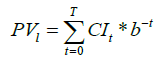
With respect to the ongoing rotation the present value of cutting incomes for each alternative was assessed according to:
 (1)
(1)
where PVl =present value of cutting incomes in stand l, l=1,..20, € ha-1, CIt =cutting income of a clear cut at year t, valued at stumpage, € ha-1 b = discount rate, b=1/(1+r) where r refers to the interest rate (here 2% or 4%) and t = time after the start of the simulation, years (T indicates time for clear cut), note that here t=T=0.
Since the biological age of the stands ranged from 60 to 160 years (Table 1), all relevant silvicultural cost can be considered to be sunk, i.e., irrelevant with respect to the time span starting from the present. Further, cutting incomes were assessed at stumpage, ignoring logging costs - the focus being on the private forest owner’s point of view. In Finland approximately 80% of the total round wood trade is based on standing sales [27].
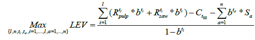
The future tree generations were assessed as follows. We started the analysis from a bare land. For both site types (MT and OMT) we applied stand-level optimization [45-47] to achieve a maximum land expectation value, Max LEV. Technically we assessed stand-level optimum for two cases for both site types, MT and OMT, representing the initial stand data. The two cases represented the northernmost and the southernmost stand, and an arithmetic average of these were finally applied as Max LEV for both site types separately. The land expectation value was maximized with respect to the number and timing of silvicultural actions and of thinnings, the intensity and type of thinnings, and rotation length. The density of seedlings per hectare was, however, adopted from the prevailing silvicultural recommendations [41]. Thus, the juvenile density was not optimized [48] but was exogenously given as described above. With application of the Faustmann’s formula [49], the LEV was maximized according to:
 (2)
(2)
where Rpulp = cutting revenues (valued at stumpage) from pulpwood removal, € ha-1;Rsaw = cutting revenues from sawlogs’ removal, € ha-1; b = discrete time discount factor, b = (1+r)-1 where r is interest rate (here, 2%, 3%, 4%); ti=timing of thinning or clear cut, years from the stand establishment, t00 (tl refers to timing for clearcut-i.e. full rotation); Ct00=stand establishment costs (incl. site preparation and planting or direct sowing) in year t00, € ha-1; ta = timing of a silvicultural action Sa (ta < ti); and Sa = individual silvicultural action (such as mounding and precommercial thinning).
For stand-level optimization we applied the optimization subroutine PIKAIA, which is part of public-domain software utilizing a genetic algorithm [50,51]. In general, genetic algorithms are more effective to find the global optimum than, e.g., direct search algorithms, and they have proved to be a useful method for solving various optimization problems [52]. The main advantages of genetic algorithms are their high precision, shorter calculations time [52] and the ability to avoid local optima [53]. Ahtikoski et al. [46,54] have described in detail the application of PIKAIA algorithm in stand-level analyses when tree growth is predicted by Motti stand simulator-as is the case here.
Finally, the differences with respect to absolute value of Max LEV between management schedules (the BAU management, and 10 and 30 year conservation) generate from the fact that the Max LEV is discounted from different time spots due to different management regimes of the ongoing rotation.
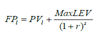
For each stand l and projection period the financial performance, FPl was calculated by summing up the results of the ongoing rotation (PVl) and the discounted value of the maximum land expectation value (Max LEV) reflecting the future tree generations:
 (3)
(3)
where FPl is the financial performance (€ ha-1), PVl is eq. (1), and Max LEV is eq.(2) and s expresses the time lag from the present to the end of the ongoing rotation, i.e. time to clear cut. The BAU management was set as the base line to which other alternatives (temporary protection for 10 or 30 years) were compared to with respect to financial performance, PVl. Then, ecological responses (CWD index and the amount of dead wood) of 10 and 30-year conservation period were based on comparing the values to initial ecological conditions of the 20 forest sites.
Optimization
Through optimization the effect of conservation target (either a) to enhance CWD index or b) to increase the amount of dead wood) on costefficiency could be demonstrated. The underlying idea (a hypothesis) was that if conservation target (a or b) did not have any effect on costefficiency, then the optimal solutions would be identical, regardless of the conservation target. An optimization task was formed according to the following steps. First, we assumed that ecological conditions (CWD index and the amount of dead wood) at the start, when the decision to clear cut or to conserve is being made, correspond to the measured values of the 20 forest sites (Table 1). Then, a hypothetical landscape was constructed consisting of those 20 forest sites. It should be emphasized that since we are only interested in proportionate (%) values, it does not matter which absolute acreage (e.g., in hectares) a single forest site, and further a landscape, presents at the start as far as the acreage of each site is identical [55]. In other words, identical optimal solutions apply regardless of the absolute acreage of a single forest site. For illustrative purposes we chose that each forest site corresponds to a one hectare, resulting in a 20 hectare landscape. The above-mentioned hypothetical landscape was chosen to simplify the interpretation of the optimal solutions: it would be easier to relate the results with a concrete physical area rather than with values expressed in merely relative terms. Finally, the discounted sum of income losses, associated with temporal conservation of 10 or 30 years, were minimized by optimization when achieving a particular conservation target. For the sake of legibility there were only two conservation targets: 1) to double the initial sum of CWD index, and 2) to double the initial amount of dead wood during the conservation period. The optimization task was simulated and solved for both conservation periods (10 and 30 years) and with two discount rates (2% and 4%).
For each forest site l a weight (wl) was determined during the optimization so that in the optimal solution the weight would correspond to a proportionate area (%) which that particular forest site presents relative to the total landscape area (denoted as 100%). The constraints presented in Eq (5) and Eq (6) illustrate the conservation targets for CWD index and the amount of dead wood, respectively. Equation (7) ensures that the total landscape adds up to 100% which here presents a 20 hectare landscape in absolute terms. Analytically, the optimization task was:
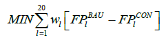 (4)
(4)
s.t.
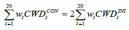 (5)
(5)
or
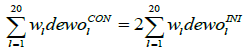 (6)
(6)
with
 (7)
(7)
where FPl BAU= financial performance (Eq. (3)) for forest site l when Business-as-usual, BAU management is applied, l=1,…, 20 , € ha-1; FPl CON= financial performance for forest site l, when the site is conserved for 10 or 30 years, € ha-1; CWDl CON= CWD index for forest site l at the end of conservation period (either 10 or 30 years); CWDl INI= initial, measured CWD index for forest site l at the start (Note that “2” refers to doubling the initial CWD index); dewol CON= the amount of dead wood for forest site l at the end of conservation period (either 10 or 30 years); dewol INI= initial, measured CWD index for forest site l at the start wl= proportional weight for forest site l relative to total landscape area, %
We applied a nonlinear solving method in the optimization due to nonlinear relations between financial performance and ecological responses [55]. Technically, the optimization was carried out using Solver tool embedded in Microsoft Excel, and the nonlinear generalized reduced gradient method (GRG2) was applied as the solving method. Finally, the optimal solutions provide weights (wl) for forest sites (l) indicating their proportionate shares of the total landscape area (100%). According to these weights of the optimal solution the conservation target (a or b) is achieved with minimized costs, keeping the total landscape area intact, here 20 hectares. Principally, the optimal solution reveals what kind of forest sites are the most cost-efficient in achieving a particular conservation target. The rationale of optimization was to find out whether there would be forest sites which dominate in the solutions, and further to analyze the underlying characteristics of these forest sites.
Sensitivity analyses
Since only two conservation targets were applied in the main analyses, alternative conservation targets were constructed in the sensitivity analyses. For a 10-year conservation period a new target was set: to increase the initial dead wood by 50%. Then, for a 30-year conservation period the new target was to triple (300%) the initial CWD index.
Results
Stand projections: Growth and yield including dead-wood volume and CWD index development
The development of each stand was predicted by the Motti stand simulator. Deadwood volume includes both the dead wood (dead standing stems and logs) in the initial state and the mortality that occurs during the conservation period, either 10 or 30 years, taking into consideration the decaying of the dead trees. In most of the sites the stand volume and the dead-wood volumes increased abundantly when conservation period was increased from 10 to 30 years (Table 1). However, there were cases in which the initial amount of dead wood even decreased when conservation period got longer (Table 1: site numbers 3, 124 and 129).
The annual mortality was 1.8% (range 0.9-2.7%) when using Siipilehto’s models. The results seem reasonable with respect to study by Peltoniemi and Mäkipää [56] which showed 1.2% mortality (range 0.2-3.3%) among nearly natural spruce dominated stands. Siipilehto’s models included both competition-related regular mortality and disturbance-related irregular mortality alike the models by, e.g., Friedman and Ståhl [57] and Monserud and Sterba [44]. On average the mean annual increment (MAI) was ca. 4.73 ha-1 year-1 during 10-yr conservation, and 4.8 m3 ha-1 year-1 during 30-yr conservation (Figure 1). However, for two forest sites the natural mortality was higher than tree growth resulting in a negative MAI values which also affect to the averages for 10-30 years (Figure 1).

Figure 1: Predicted (by Motti stand simulator) mean annual increments, MAIs, by forest sites for 10-year and 30-year conservation periods, m3 ha-1 year-1. Numbers on x axis refer to site numbers (Table 1).
The CWD index development during conservation is presented in Figure 2. It can be easily depicted that in each forest site CWD index increased towards to the 30-year conservation period (Figure 2). For instance, in forest site number 157 the initial CWD index was 0, but it increased up to 18 within 30 years (Figure 2).

Figure 2: Development of the CWD index by forest sites, index value (y axis) is a plain number. Numbers on x axis refer to site numbers.
According to the simulations the amount of dead wood on average increased from 25.1 m3 ha-1 (at the start) to 41 m3 ha-1 and to 71.3 m3 ha-1 when the conserving 10 or 30 years, respectively (Figure 3). Furthermore, in some sites the increase of the amount of dead wood was distinctive: the amount of dead wood at the end of 30-year conservation was over 20 times the initial amount of dead wood (Figure 3). In brief, temporary conservation has enhanced considerably both the CWD index and the amount of dead wood in our study sites.

Figure 3: The amount of dead wood at the start and after 10-year and 30-year conservation periods, m3 ha-1. Numbers on x axis refer to site numbers.
Financial performance
The income losses expressed as differences in financial performance between BAU management and fixed-term conservation alternatives (see Eq.(3) for technical details) fluctuated considerably. For instance, with 4% discounting the income losses ranged from 165 up to 10 900 € ha-1 when the conservation period was 10 years (Figure 4). With 2% discounting the income losses varied between 309 and 17700 € ha-1 when conservation period was 30 years (Figure 4).

Figure 4: Income losses associated with 4% discounting and 10-year conservation period and 2% discounting and 30-year conservation period, € ha-1. Numbers on x axis refer to site numbers.
Optimization
As anticipated, optimal allocation of forest sites differed depending on the conservation target when conservation period was 10 years (Table 2). For instance, when the conservation target was to double the initial amount of dead wood, the two most cost-efficient forest sites to achieve this target were site numbers 3 and 129, when discounting with 2% (Table 2). When the conservation target was to double the initial CWD index then the two most cost-efficient forest sites were site numbers 109 and 129 (Table 2). The main result regarding the 10-year conservation period was that forest site 129 was included in the optimal solution regardless of the conservation target or discount rate (Table 2).
| Site number | Initial values | Discount rate 2% | Discount rate 4% | Sensitivity analysis*** | |||||
|---|---|---|---|---|---|---|---|---|---|
| Volume* | Dead wood* | CWD index* | 2 ×dewo** | 2 × CWD ** | 2×dewo | 2×CWD | 2% | 4% | |
| 1_2 | 348 | 7.2 | 12 | ||||||
| 1_3 | 406 | 34.6 | 19 | ||||||
| 2 | 509 | 69.1 | 39 | ||||||
| 3 | 200 | 147.3 | 23 | 12% | 12% | ||||
| 4_4 | 482 | 23.7 | 23 | ||||||
| 4_6 | 749 | 41.3 | 26 | ||||||
| 101 | 382 | 7.2 | 22 | ||||||
| 102 | 436 | 13.8 | 20 | ||||||
| 104 | 441 | 2.5 | 7 | ||||||
| 109 | 337 | 12.3 | 29 | 85% | 69% | ||||
| 202 | 669 | 8.6 | 3 | ||||||
| 216 | 511 | 22.1 | 11 | ||||||
| 219 | 332 | 4.7 | 11 | ||||||
| 124 | 108 | 32.1 | 12 | 5% | |||||
| 129 | 211 | 39.5 | 16 | 88% | 15% | 88% | 31% | 99% | 95% |
| 157 | 395 | 0 | 0 | ||||||
| 176 | 367 | 0.8 | 1 | 1% | |||||
| 180 | 390 | 14.3 | 8 | ||||||
| 221 | 291 | 13.3 | 9 | ||||||
| 260 | 378 | 6.8 | 17 | ||||||
| average | 397.1 | 25.1 | 15.4 | ||||||
Table 2: Optimal solutions reflecting the most cost-efficient allocation among sites (expressed in % of total landscape) when conservation period is 10 years. Conservation target either to double the initial amount of dead wood (2 x dewo) or to double the initial CWD index during the 10-year conservation period (2 x CWD). Discount rates 2% and 4%.
Two forest sites (numbers 124 and 129) dominated the optimal solutions when the conservation period was 30 years - regardless of the conservation target or discount rate (Table 3). However, also forest site number 3 was included in those two optimal solutions, but not as a majority (Table 3). When analyzing the optimal solutions of 10 and 30-year conservation periods together, one can argue that forest site numbers 124 and 129 dominate the optimal solutions implying that they might be the most cost-efficient sites, particularly for 30-year conservation – regardless of the conservation target. The answer for the superiority of forest site numbers 124 and 129 can be found by studying the initial characteristics as well as simulated results of growth and yield, decaying wood as well as income losses. First and foremost, the income losses associated with forest site numbers 124 and 129 are the lowest (Figure 4) which partly originates from the fact that the mean annual increments are above average (Figure 1)and partly due to distinctively below-average initial stand volume (Table 1). The latter (below-average stand volumes) indicates that there is a growth potential allocative to saw logs rather than pulpwood still availablethus, postponing immediate clear cut by conserving the sites actually increases the cutting incomes when discounting with low interest rates such as 2%. Further, initial dead wood of forest site numbers 124 and 129 is well above the average, but CWD index more or less the average of the 20 forest sites of the study. The ecological responses for forest site numbers 124 and 129 present slightly below (129) or above (124) the averages among the 20 forest sites of the study (see Figure 3 for dead wood and Figure 2 for CWD index development). Finally, combining the distinctively low income losses with more or less average ecological responses results in an incomparably cost-efficient forest sites for conservation-at least among the 20 forest sites included in this study. However, the forest sites that are most cost-efficient for temporary conservation are not necessarily ecologically the most valuable ones.
| Siten number | Initial values | Discount rate 2% | Discount rate 4% | Sensitivity analysis* | |||||
|---|---|---|---|---|---|---|---|---|---|
| Volume | Dead wood | CWD index | 2 × dewo | 2 × CWD | 2 × dewo | 2 × CWD | 2% | 4% | |
| 1_2 | 348 | 7.2 | 12 | ||||||
| 1_3 | 406 | 34.6 | 19 | ||||||
| 2 | 509 | 69.1 | 39 | ||||||
| 3 | 200 | 147.3 | 23 | 20% | 31% | ||||
| 4_4 | 482 | 23.7 | 23 | ||||||
| 4_6 | 749 | 41.3 | 26 | ||||||
| 101 | 382 | 7.2 | 22 | ||||||
| 102 | 436 | 13.8 | 20 | ||||||
| 104 | 441 | 2.5 | 7 | ||||||
| 109 | 337 | 12.3 | 29 | ||||||
| 202 | 669 | 8.6 | 3 | ||||||
| 216 | 511 | 22.1 | 11 | ||||||
| 219 | 332 | 4.7 | 11 | ||||||
| 124 | 108 | 32.1 | 12 | 25% | 69% | 25% | 92% | 92% | |
| 129 | 211 | 39.5 | 16 | 80% | 75% | 75% | 8% | 8% | |
| 157 | 395 | 0 | 0 | ||||||
| 176 | 367 | 0.8 | 1 | ||||||
| 180 | 390 | 14.3 | 8 | ||||||
| 221 | 291 | 13.3 | 9 | ||||||
| 260 | 378 | 6.8 | 17 | ||||||
| average | 397.1 | 25.1 | 15.4 | ||||||
Table 3: Optimal solutions reflecting the most cost-efficient allocation among sites (expressed in % of total landscape) when conservation period is 30 years. Conservation target either to double the initial amount of dead wood (2 x dewo) or to double the initial CWD index during the 10-year conservation period (2 x CWD). Discount rates 2% and 4%. See Table 2 for full variable names (in columns).
Discussion
Fulfilling conservation policy targets means increased protection of forest biodiversity implying reduced income from timber production for private forest owners [7]. Thus, it is utmost relevant to examine the cost-efficiency related to alternative approaches of biodiversity conservation in forests. This study focused on relatively new approach to enhance biodiversity in forests-temporal conservation [6]. Further, we demonstrated by a hypothetical landscape and through optimization whether the conservation goal has any impact on costefficiency. Another rationale for optimization was to find out possible high-performing forest sites (i.e., the most cost-efficient) which would stand out from the mass, and further to analyse these with respect to both ecological (amount of dead wood and CWD index) ) and financial (income losses) variables.
Many red-listed species occur only in later decay classes of dead wood [58] implying that the amount of dead wood itself might not be a sufficient indicator for conservation purposes. Current practices, for instance in Finland, indicate that both the amount and quality of dead wood are important factors when choosing suitable stands for conservation. Another relevant aspect related to conservation in commercial forests is time: does the length of conservation contracts matter with respect to cost-efficiency and ecological outcome [11]. Our study tackled with both issues: the amount of dead wood and the length of conservation contracts. Contradicting to earlier studies, we focused solely on a stand level so that income losses and ecological responses due to temporal conservation were compared. The stand projections (including decaying wood cohorts and decay stages) produced by Motti stand simulator were by technical design and execution identical to those reported in Juutinen et al. We consider that the forecasted development by Motti stand simulator for 10 and 30-year conservation period was realistic with respect to relevant variables such as growing stock and the amount of coarse woody debris, CWD.
Earlier studies revealed that in voluntary biodiversity conservation contracts an average demand for financial compensation (i.e., to compensate the income loss due to temporal conservation) was around 200 € ha-1 annually [59]. For cost of producing dead wood our results suggest income losses within a range of ca. 90 to 200 € m-3 (Table 1) (Figure 3), and for enhancing CWD index the cost range was from ca. 400 to 1500 € per one unit increase in CWD index (Figures 2 and 3), depending on the discount rate and conservation period. Note that the increase of the amount of dead wood or CWD index during the contract period does not extensively describe the ecological value of the site. On the sites that have high CDW index and above-average initial amount of dead wood already in the beginning of the conservation period, the increase of these factors can be more moderate than on the sites where the level of CWD index and amount of dead wood is noticeably lower in the beginning. A site with higher CWD index and amount of dead wood can be ecologically more valuable-even there would not be any increase in these factors during the contract period -than a site where the increase is higher but that does not reach the same level. Although these results cannot be directly compared to earlier studies in similar climatic conditions, our results are in line with them representing alike magnitude of conservation costs [59].
Despite applying a hypothetical landscape and imaginary conservation targets the main results can conclusively be interpreted with relevancy to real-world situations. Namely, conservation target does matter-the optimal allocation of forest sites to achieve particular target with least costs (i.e., the most cost-efficiently) changed along with the target. Simply, each optimal solution was-at least-slightly different than another. In this connection it is worth emphasizing again that theoretically it did not matter had we applied different absolute acreages for each of the 20 forest sites in this study. This is due to the fact that optimization was technically solved by using proportional (%) instead of absolute scale [55].
The importance of conservation target on cost-efficiency shown here has a clear signal to practical decision-makers: the conservation target needs to be well-defined before assessing the cost-efficiency of the conservation. The forest sites with distinctively above-average initial amount of dead wood and excellent growth potential (indicating lower than average income losses) shone through with respect to costefficiency. The length of conservation period has an impact to the results, too.
From the decision-making point of view our results are intriguing. Principally, the conservation of biodiversity provides public goods, the benefit of which cannot be exclusive to the private forest owner [59]. It can be argued that the owner should be compensated for all the lost private values when the resource is used to produce public services, provided that land ownership is complete and exclusive [60]. Bearing that in mind, the results of this study can be interpreted as following. If there are no constraints regarding the decision (i.e., rational and free choice opportunity, no budget constraint), if the forest owner is not going to cut the stand after the expiry of the contract and compensation is solely derived from the income loss during the contract period, then private forest owners should aim at choosing 30-year conservation period over 10-year period since longer conservation periods yield higher absolute compensation values (€), regardless of the ecological targets. On the other hand, longest available conservation periods are not necessary the most cost-efficient from the financier’s point of view (e.g., government), nor are they inevitably the best for improving biodiversity. Longer conservation period for a less ecologically valuable site may reduce financial possibilities to make contracts for alternative, more ecologically valuable sites. This creates a problem in which private forest owners and general conservation targets might conflict. Basically, the solution for such a problem depends on the budget constraint (how much money is available for compensating private income losses) and particular conservation targets in general (desirable level of biodiversity expressed e.g. as the amount of red-listed species or aggregate CWD index).
The most cost-efficient sites are not necessarily the ones that are biologically most valuable and therefore the desirable level on biodiversity might not be fulfilled by choosing merely the most costefficient sites. Furthermore, the policy makers need to consider several different attributes which eventually describe the complex characteristics of biodiversity. One option might be to apply habitat suitability index [7,11] or to estimate through specific models the amount of red-listed species (the models being based on the CWD index), or to apply other measures [2] to rank suitable stands for conservation.
References
- Anonymous (1999) World Commission on forests and sustainable development. Our forests our future. Report of the World Commission on forests and sustainable development. Cambridge University Press, Cambridge, England.
- Lindemayer DB, Franklin JF, Fischer J (2006) General management principles and a checklist of strategies to guide forest biodiversity conservation Biol Conserv 131: 433-445.
- Johansson T, Hjälten J, de JJ, Stedingk VH (2013) Environmental considerations from legistation and certification in managed forest stands: a review of their importance for biodiversity For Ecol Manage 303: 98-112.
- Niemela J, Koivula M, Kotze DJ (2007) The effects of forestry on carabid beetles (Coleoptera: Carabidae) in boreal forests J Ins Conserv 11: 5-18.
- Ekvall H, Bostedt G, Jonsson M (2013) Least-cost allocation of measures to increase the amount of coarse woody debris in forest estates J.Forest Econ 19: 267-285.
- Ando A, Chen X (2011) Optimal contract lengths for voluntary ecosystem service provision with varied dynamic benefit functions Conserv Letters 4: 207-218.
- Juutinen A, Reunanen P, Monkkonen M, Tikkanen OP, Kouki J (2012) Conservation of forest biodiversity using temporal conservation contracts Ecol Econ 81: 121-129.
- Juutinen A, Ollikainen M (2010) Conservation contracts for forest biodiversity. Theory and experience from Finland For Sci 56: 201-211.
- Ranius T, Ekvall H, Jonsson M, Bostedt G (2005) Cost-efficiency of measures to increase the amount of coarse woody debris in managed Norway spruce forests for Ecol Manage 206: 119-133.
- Comerford E (2013) The impact of permanent protection on cost and participation in a conservation programme: a case study from Queensland Land Use Policy 34: 176-182.
- Juutinen A, Ollikainen M, Monkkonen M, Reunanen P, Tikkanen OP et al. (2014) Optimal contract length for biodiversity conservation under conservation budget constraint For policy and eco 47 :14-24.
- Jonsson M, Ranius T, Ekvall H, Bostedt G, Dahlberg A et al. (2006) Cost-effectiveness of silvicultural measures to increase substrate availability for red-listed wood-living organisms in Norway spruce forests Biol Conserv 127: 443-462.
- Bergseng E, Ask JA, Framstad E, Gobakken T, Solberg B et al. (2012) Biodiversity protection and economics in long term boreal forest management-a detailed case for the valuation of protection measures For Policy Econ 15: 12-21.
- Anonymous (2008) Government Resolution on the Forest Biodiversity Action Programme for Southern Finland 2008-2016 (METSO). The Govt of Finland 15.
- Syrjänen K, Hakalisto S, Mikkola J, Musta I, Nissinen M, et al. (2016) Monimuotoisuudelle arvokkaiden metsäympäristöjen tunnistaminen METSO-ohjelman luonnontieteelliset valintaperusteet 2016-2025. Reports of the Ministry of the Environment 17/2016 .75 [Identification of forest ecosystems valuable in terms of biodiversity. Scientific selection criteria of the Forest Biodiversity Programme for Southern Finland (METSO) 2016-2025. Ministry of the Environment & Ministry of Agriculture and Forestry.
- Juutinen A, Luque S, Monkkonen M, Vainikainen N, Tomppo E (2008) Cost-effective forest conservation and criteria for potential conservation targets: a Finnish case study Environ Sci Policy 11: 613-626.
- Siitonen J, Martikainen P, Punttila P, Rauh, J (2000) Coarse woody debris and stand characteristics in mature managed and old-growth boreal mesic forests in southern Finland For Ecol Manage 128: 211-225.
- Siitonen J, Jonsson BG (2012) Other associations with dead woody material. In: Stokland, J.N., SiitonenJ, Jonsson, B.G. (Eds.). Biodiversity in Dead Wood Cambridge University Press, Cambridge, UK 58-81.
- Juutinen A, Monkkonen M, Sippola A (2006) Cost-efficiency of decaying wood as a surrogate for overall species richness in boreal forests Conserv Biol 20: 74-84.
- Harmon ME, Franklin JF, Swanson FJ, Sollins P, Gregory SV et al. (1986) Ecology of coarse woody debris in temperate ecosystems Adv Ecol Res 15: 133-302.
- Franklin JF, Shugart HH, Harmon ME (1987) Tree death as an ecological process. The causes, consequences, and variability of tree mortality Bio Sci 37: 550-556.
- Samuelsson J, Gustafsson L, Ingelog T (1994) Dying and dead trees: a review of their importance for biodiversity Swedish Threatened Spcs Unit Uppsala 109.
- Esseen PA, Ehnstrom B, Sjoberg K, Ericson L (1997) Boreal forests In: Hanson, L. (Ed.), Boreal ecosystems and landscapes: structures, processes and conservation of biodiversity Ecol Bull.46: 16-47.
- Siitonen J, Hottola J, Immonen A (2009) Differences in stand characteristics between brook-side key habitats and managed forests in southern Finland Silva Fenn 43: 21-37.
- Tonteri T, Hotanen JP, Kuusipalo J (1990) The Finnish forest site type approach: ordination and classification studies of mesic forest sites in southern Finland Vegetatio 87: 85-98.
- Laasasenaho J (1982) Taper curve and volume functions for pine, spruce and birch Comm Inst For Fenn 108: 1-74.
- Anonymous (2012-2014) Finnish Statistical Yearbook of Forestry 2012-2014. Finnsih Forest Research Institute, Helsinki.
- Hynynen J, Ahtikoski A, Siitonen J, Sievanen R, Liski J (2005) Applying the MOTTI simulator to analyse the effects of alternative management schedules on timber and non-timber production. For Ecol Manage 207: 5-18.
- Salminen H, Lehtonen M, Hynynen J (2005) Reusing legacy FORTRAN in the MOTTI growth and yield simulator Comput Electron Agric 49: 103-113.
- Hynynen J, Salminen H, Huuskonen S, Ahtikoski A, Ojansuu R, et al. (2014) Scenario analysis for the biomass supply potential and the future development of Finnish forest resources. Working Papers of the Finnish Forest Research Institute 302 106.
- Hynynen J, Ojansuu R, Hokka H, Siipilehto J, Salminen H, et al. (2002) Models for predicting stand development in MELA System. Metsäntutkimuslaitoksen tiedonantoja-The Finnish Forest Resrch Ins Research Papers 835 116.
- Matala J, Hynynen J, Miina J, Ojansuu R, Peltola H et al. (2003) Comparison of a physiological model and a statistical model for prediction of growth and yield in boreal forests Ecol Model 161: 95-116.
- Siipilehto J (2009) Modelling stand structure in young Scots pine dominated stands For Ecol Manage 257: 223-232.
- Hokka H (1997) Height diameter curves with random intercepts and slopes for trees growing on drained peatlands For Ecol Manage 97: 63-72.
- Hokka H, Salminen H (2006) Utilizing information on site hydrology in growth and yield modeling: peatland models in the MOTTI stand simulator. In Proceedings of the international conference: Hydrology and management of forested wetlands, April 8-12 2006. New Bern, North Carolina, US 302-309.
- Huuskonen S, Ahtikoski A (2005) Ensiharvennuksen ajoituksen ja voimakkuuden vaikutus kuivahkon kankaan männikoiden tuotokseen ja tuottoon Metsatieteen aikakauskirja 2: 99-115.
- Makinen H, Hynynen J, Isomaki A (2005) Intensive management of Scots pine stands in southern Finland: First empirical results and simulated further development For Ecol Manage 215: 37-50.
- Huuskonen S (2008) The development of young Scots pine stands-precommercial and first commercial thinning. Dissertationes Forestales 62.
- Monkkonen M, Juutinen A, Mazziotta A, Miettinen K, Podkopaev D, et al. (2014) Spatially dynamic forest management to sustain biodiversity and economic returns. J of Environ management 134: 80-89.
- Hynynen J, Salminen H, Ahtikoski A, Huuskonen S, Ojansuu R, et al. (2015) Long-term impacts of forest management on biomass supply and forest resource development: a scenario analysis for Finland European J of Forest Research 134: 415-431.
- Aijala O, Koistinen A, Sved J, Vanhatalo K, Vaisanen P (2014) Metsanhoidon suositukset. [Finnish silvicultural guidelines]. Metsätalouden Kehittämiskeskus Tapio. Metsäkustannus, Helsinki. 150 p + Appendices [in Finnish].
- Haapala P (1983) Luonnonpoistuman ennustaminen puun kuolemistodennäköisyysmallilla. Metsäntutkimuslaitoksen puuntuotoksen tutkimussuunta[Estimating the mortality according to propability functions, growth and yield studies of Finnish Forest Research Institute] Stencil 33 [in Finnish]
- Monserud R (1976) Simulation of forest tree mortality For Sci 22: 438-444.
- Monserud R, Sterba H (1999) Modelling individual tree mortality for Austrian forest species For Ecol Manage 113: 109-123.
- Niinimaki S, Tahvonen O, Makela A (2012) Applying a process-based model in Norway spruce management For Ecol Manage 265: 102-115.
- Ahtikoski A, Salminen H, Ojansuu R, Hynynen J, Karkkainen K (2013) Optimizing stand management involving the effect of genetic gain: preliminary results for Scots pine in Finland Can J For Res.43: 299-305.
- Ramo J, Tahvonen O (2017) Optimizing the harvest timing in continuos cover forestry Environ Resource Econ 853-868.
- Hyytiainen K, Tahvonen O, Valsta L (2005) Optimum juvenile density, harvesting and stand structure in even-aged Scots pine stands For Sci 51: 120-133.
- Faustmann M (1849) Berechnung des Werthes, welchen Waldboden, sowie noch nicht haubare Holzbestände für die Waldwirthschaft besitzen. [Calculation of the value which forest land and immature stands possess for forestry]. Allgemeine Forst- und Jagd-Zeitung 25: 441-455.
- Charbonneau P, Knapp B (1995) A user’s guide to Pikaia 1.0, NCAR Technical Note 418+IA. High Altitude Observatory, National Center for Atmospheric Research, Boulder, Co.
- Charbonneau P (2002) An introduction to genetic algorithms for numerical optimization, NCAR Technical Note TN-450+IA. High Altitude Observatory, National Center for Atmospheric Research, Boulder, Co.
- Li MJ, Chen DS, Wang F, Li Y, Zhou Y et al. (2010) Optimizing emission inventory for chemical transport models by using genetic algorithm Atmos Environ 44: 3926-3934.
- Hadi MRHS, Gonzalez AJL (2009) Comparison of fitting weed seedling emergence models with nonlinear regression and genetic algorithm Comput Electron Agric 65: 19-25.
- Ahtikosk A, Salminen H, Hokka H, Kojola S, Penttila T (2012) Optimizing stand management on peatlands: the case of northern Finland Can J For Res 42: 247-259.
- Bazaraa MS, Sherali HD, Shetty CM (2006) Nonlinear programming, theory and algorithms. 3rd Edition. Wiley-InterScience, A John Wiley & Sons, Hoboken, NJ 853.
- Peltoniemi M, Makipaa R (2010) Quantifying distance-independent tree competition for predicting Norway spruce mortality in unmanaged forests For Ecol Manage. 261: 30-42.
- Friedman J, Stahl G (2001) A three-step approach for modelling tree mortality in Swedish forests Scan J For Res 16: 455-466.
- Tikkanen OP, Martikainen P, Hyvarinen E, Junninen K, Kouki J (2006) Red-listed boreal forest species in Finland: associations with forest structure, tree species, and decaying wood Ann Zool Fenn 43: 373-383.
- Horne P (2006) Forest owners acceptance of incentive based policy instruments in forest biodiversitEnly conservation - a choice experiment based approach. Silva Fenn 40: 169-178.
- Innes R, Polasky S, Tschirart J (1998) Takings, compensation and endangered species protection on private lands J Econ Perspect 12: 35-52.