Spanish
  Chinese
  Russian
  German
  French
  Japanese
  Portuguese
  Hindi
Hindi Research Article, Res J Econ Vol: 7 Issue: 5
Econometric Analysis of Exchange Rates on Current Account Adjustments in Rwanda
Ibrahim Osman Sesay*
Department of Administrative, Kamet Turbo Engineering Limited, Greater Accra, Ghana
- *Corresponding Author:
- Sesay IO
Department of Administration and Management,
Kamet Turbo Engineering Limited,
Greater Accra,
Ghana;
E-mail: ibrahimosmansesay@gmail.com
Received date: 11 May, 2023, Manuscript No. RJE-23-105533;
Editor assigned date: 16 May, 2023, PreQC No. RJE-23-105533
(PQ);
Reviewed date: 30 May, 2023, QC No. RJE-23-105533;
Revised date: 14 June, 2023, Manuscript No. RJE-23-105533 (R);
Published date: 12 July, 2023, DOI: 10.4172/RJE.1000156
Citation: Sesay IO (2023) Econometric Analysis of Exchange Rates on Current Account Adjustments in Rwanda. Res J Econ 7:4.
Abstract
In this work, we use the Vector Auto-Regression (VAR) model to analyze the determinants driving the exchange rate and current account balance of Rwanda, based on BNR quarterly macroeconomic time series data from 2000 Q1 to 2020 Q4. The trade balance is the dependent variable and the real effective exchange rate, GDP per capita, trade openness, trade conditions and Foreign Direct Investment (FDI) are the explanatory factors. The data were transformed into natural logarithms. According to our findings, all variables at I are stationary, which means that there is a long-run relationship between the cointegrating variables. The results of the linear model show that the real effective exchange rate has no impact on the trade balance in the short run but improves the trade balance in the long run. In addition, Granger causality and impulse response analyzes are used to study the dynamics of exchange rates and current account adjustments. Examining the VAR impulse responses for Rwanda, we detect external demand and supply shocks. We also provide evidence of spillover effects from Rwandan demand shocks and central interest rate policy shocks. This study recommends to policymakers that the devaluation of the Rwandan franc improves the trade balance in the long run, all things being equal, whereby an increase in Foreign Direct Investment (FDI) in Rwanda could lead to increased Rwandan economic investment, which would improve Rwanda's current account balance. However, it must be noted that the increase in the volume of foreign direct investment in Rwanda also increases imports and repatriation
Keywords: Current account, Exchange rate, Monetary policy, Foreign Direct Investment (FDI), Vector Auto-Regression (VAR)
Introduction
Background of the study
The current account is one of the components of the balance of payments, along with other components such as the capital account, financial account, reserve account and net error and omission account.
The balance of payments records all the financial transactions that a country conducts with other countries in a year. These transactions allow the transfer of ownership of anything that has economic value and can be expressed in money from the citizens of one country to the citizens of the other country. International transactions are documented in the balance of payments for reasons of double-entry bookkeeping, in which each transaction is increased by two counter-postings with the same value, so that conceptually the postings that cause it on both sides are always the same. Transactions are normally respected at market cost and are recognized whenever possible when a change of ownership occurs. Transactions related to products, services and unilateral transfers are recorded in the current accounts and transactions related to liabilities and financial assets are recorded in the capital accounts. In theory, policymakers have two options for improving the country's trade balance and changing the country's competitiveness. The internal approach is based on supply-side policies, such as influencing labor productivity or wages by lowering inflation, lowering taxes or loosening labor market conditions. The external approach, on the other hand, consists of depreciating the currency [1].
The relationship between REER and trade balancing has been studied in a number of empirical studies with varying degrees of success. According to one line of research, there is a consistent relationship between REER and trade balance. According to the empirical model of Oskoees, after currency depreciation, the trade balance initially deteriorates due to the lag structure of exchange rates, but eventually improves over time. Schaling and Kabundi examined this pattern and found that real depreciation ultimately improves the trade balance between South Africa and the US, supporting the Jcurve phenomenon. The exchange rate is then the value of one currency in relation to another. For example, the current exchange rate from pounds to dollars is 1 pound=1.2 US dollars. This means that it takes 1 pound to buy a product worth $1.6. And from a dollar perspective, that means $1.2 can buy £1 worth of goods and services. Devaluation of a currency means that the value of the currency decreases in terms of another currency. This means that the country will have to pay more to buy goods and services that it buys from other countries. And if the currency value appreciates, this means that the country will have to now pay less to buy the same amount goods and services. Devaluation leads to decrease in the purchasing power of the currency and appreciation lead to the increasing purchasing power of the currency. The current account records transaction of products, services and unilateral transfers between residents of one country and the other. It is one of the measures to calculate the country’s foreign trade.
The current account consists of the following four components such as goods: Being portable and physical in characteristics, products are often exchanged by nations all over the world. When a deal of certain good's possession from a nation to overseas occurs, this is called an "export."
Services: When an intangible service (e.g. tourism) is used by a foreigner in a regional area and the regional citizen gets the cash from a foreigner, this is also mentioned as a trade, thus a credit score [2].
Income: A credit score of earnings happens when a personal or an organization of household nationality gets cash from a organization or personal with international identification. An international organization's investment upon a household organization or a municipality is considered as a credit score. Formula of the calculate the current account balance: Current account=(X-M)+NY+NCT.
X=Exports, M=Imports, NY=Net income abroad, NCT=Net Current Transfer
Rwanda ran a sizeable and persistent current account deficit during the period, mainly due to the goods trade deficit. This goods trade deficit is the result of higher imports versus flat and less diverse exports. Despite this persistent trade deficit, little attention has been paid to the size of Rwanda's trade elasticities. Nuwagira and Muvunyi examined the presence of the Marshall-Lerner condition, i.e. the need for depreciation to improve the trade balance and noted that the condition exists.
Nexus between current account movements and exchange rate in Rwanda
The relationship between exchange rates and current account balance is strong. The balance of payments is heavily influenced by exchange rates. When a country's exchange rate falls, the value of its currency relative to another country falls, making its exports cheaper and its imports more expensive. This can lead to a current account deficit and a negative balance of payments. On the other hand, an increase in the exchange rate of a currency will help the country improve its current account balance and hence its balance of payments. More broadly, developments in Rwanda's trade deficit and real effective exchange rates. The consumer price index is used to calculate the real effective exchange rate for Rwanda's 10 trading partners (CPI). Depreciation is indicated by an increase in the exchange rate and vice versa. Over the past two decades, Rwanda has maintained a current account deficit, mainly driven by the trade deficit, which exceeds significant inflows from official and private transfers. Strong imports, needed to meet domestic demand for consumption and investment, along with sluggish and less diverse exports have contributed to the widening trade deficit. However, Rwanda has recently implemented a series of initiatives known as Made in Rwanda to diversify its export base, particularly adding value to its conventional raw materials, and to strengthen Rwanda's manufacturing base (Figure 1).

Figure 1: Current account and real effective exchange rate in Rwanda from 2000Q1 to 2020Q2.
Over the years 2000-2020, real effective exchange rates increased in 2000, 2006, 2019 and 2020 on average and current account reduce from 2018 due to unfavorable trade between Uganda and Rwanda and 2020 due to COVID 2019 outbreak, Kharroubi stated that when a country is vertically specialized, its exports depend greatly on the number of imports. As a result, the trade balance responds to a change in the real exchange rate less quickly when imports and exports move together more closely (Figure 2) [3].

Figure 2: Current account and others macroeconomic indicator.
Over 20 years from 2000, the evolution of Rwanda's trade deficit is mainly caused by the trade deficit and outpaces significant inflows from official and private transfers. Strong imports required to meet domestic demand for consumption and investment, combined with sluggish and less diverse exports, have contributed to the rising trade deficit.
Conceptual framework
The primary aim of this research is to contribute to the econometric analysis of the exchange rate for current account adjustment in Rwanda. The country of Rwanda was chosen for two reasons. First, there are few empirical studies that have examined the relationship between Rwanda's exchange rate and trade balance. To our knowledge, no study on the relationship between the real exchange rate and the trade balance has been conducted, apart from the three previous studies that examined the effects of the exchange rate on exports and imports separately. Second, previous studies of trade elasticities in Rwanda relied on linear models that assumed an asymmetric effect of the real exchange rate on trade flows. Therefore, this working paper aims to answer questions such as: B. What is the impact of the real effective exchange rate on the impact on the trade balance. To study the spillover effect on demand and supply shocks to determine the effect of (independent) orthogonality variabales such as real effective exchange rate (reer), GDP per capita (GDP_Ca), Trade Openness (TR), trade conditions determine (TOT) and Foreign Direct Investment (FDI) on current account of Rwanda.
This conceptual framework of our study in Figure 3 gives blue print that taking into account dependent variable such as the real effective exchange rate (reer), GDP per capita (GDP_Ca) trade openness (TR), Terms of Trade (TOT) and Foreign Direct Investment (FDI) and dependent variable such as trade balance and finally intervening variables such as foreign policy and domestic policy in form of Inflation shock, financial shocks, monetary policy shocks and demand shocks.

Figure 3: Conceptual framework.
Theoretical literature
Several empirical research has examined the causes and effects of current account adjustment. Milesi-Ferretti and Razin were the first to do so methodically, applying Eichengreen, Rose and Wyplosz's methodology from currency crises to current account adjustments. The Asian crisis of 1997-1998 inspired Milesi-Ferretti and Razin to focus on low- and middle-income countries. Using a set of empirical criteria, the authors identify multiple adjustment episodes ("reversals") and discover that somewhat more than half of them are connected with an economic slowdown. Using a probit analysis, they find that adjustments are more likely in countries with large current account deficits, lower reserves, higher GDP per capita, worsening terms of trade, an increasing investment rate and floating exchange rate. Two external variables, namely BNR growth and the US interest rate, also turn out to be robust predictors of adjustment.
This approach was extended to industrial countries by Freund. Using a dataset of 25 adjustment episodes during 1980-1997, she finds that average adjustments start when the current account deficit reaches 5 percent of GDP. Slowing income growth and a real depreciation of about 10 to 20 percent are the major drivers of adjustment. Strengthening real export growth, decreasing investment growth and a levelling off in the budget deficit are also part of the adjustment process. These findings suggest that current account adjustments in industrial countries are largely manifestations of the business cycle. Freund’s probit analysis fails to identify good predictors of current account reversals, leading the author to conclude that the exact timing of an adjustment is very difficult to forecast (Figure 4).

Figure 4: Exchange rate (GDP/Capita).
Adalet and Eichengreen’s samples goes back to the gold standard of the late-19th century. They find that adjustments were more frequent in recent history (post-Bretton Woods era) than in earlier historical episodes. Also de Haan et al. and IMF use somewhat longer samples than the rest of the literature, starting in 1960. In this paper, we will restrict the sample to the post-Bretton Woods era, starting in 1973.
Role of financial variables and sudden stops. Several authors have sought to bridge the literature on current account adjustments with that on sudden stops. Sudden stops refer to abrupt and large reductions in capital inflows and have been studied inter alia by Calvo et al. and Calvo and Talvi. Edwards finds that sudden stops, in the presence of large current account deficits, increase the likelihood of a current account adjustment. De Haan et al. show that a higher degree of financial openness lowers the probability of current account adjustment in BNR countries. Freund and Warnock study the composition of financial flows but do not find a systematic relation with current account adjustments. Also Debelle and Galati examine the role of financial flows, highlighting that financial account variables help explain why countries run a large current account deficit, but not why they go through a current account adjustment.
Adjustment in developing and emerging market economies. A number of papers focus mainly on developing and emerging market economies, including the seminal work of Milesi-Ferretti and Razin, the comparison of Asia’s and Latin America’s experience by Guidotti et al., and the studies of transition economies. In this paper, we focus on industrial economies and the most advanced emerging market economies [4].
Empirical literature
The diversity across adjustment episodes is generally acknowledged in the literature. Only few authors, however, have explicitly addressed it by distinguishing subgroups of adjustment.
Distinction between low-growth and high-growth adjustment. Croke, Kamin and Leduc and IMF select among their industrial country episodes the top and the bottom performers in terms of real GDP growth. Croke, Kamin and Leduc find that the low-growth cases are not characterized by significantly higher volatility in exchange rates, interest rates or share prices. The IMF finds that low-growth cases tend to exhibit a relatively modest degree of real effective depreciation, whereas high-growth cases were associated with aboveaverage real depreciation.
Distinction between export-led and import-driven adjustment. Guidotti et al. investigate differences in export and import performance during adjustments in emerging market and developing economies. They conclude that stronger export growth was the main driver of adjustment in emerging Asia while slowing import growth was the main driver in Latin America. The authors attribute this difference to structural factors, highlighting that more closed economies and economies with a higher degree of liability dollarization are more likely to adjust through import contraction. Distinction between large and small countries. Edwards finds that the harmful effects of current account adjustment on economic growth tend to be more significant for larger countries.
Distinction in terms of adjustment threshold. Clarida, Goretti and Taylor identify country-specific thresholds for current account adjustment, i.e. levels of the current account to output ratio above which the current account tends to revert to equilibrium. Applying their methodology to G7 countries, they find that thresholds differ significantly across countries, ranging on the deficit side from 0.18 percent in Japan to 4.05 percent in Canada.
These papers highlight that adjustments have different implications for macroeconomic and financial stability. The central contribution of this paper is to assess the diversity across episodes in a systematic way, in terms of both the adjustment dynamics and the developments before the start of the adjustment. Before presenting the results, the following section reviews the data and the episode selection [5].
Materials and Methods
Stationary time series
If the mean and auto covariance of the series do not vary on time, the series is considered to be (weakly or covariance) stationary. Nonstationary refers to any series that is not stationary.
The random walk is an illustration of a non-stationary series that is as follow:
Where, εt is a stationary random disturbance term; the series Yt has a constant forecast value, conditional on t; and the variance is increasing over time. Augmented Dickey-Fuller (ADF), Phillips- Perron test (PP), GLS detrended Dickey-Fuller (ERS), KPSS and Ng- Perron tests (NP) are recognized as unit root tests for a time series to be stationary or not. The random walk is a difference stationary series, since the first difference of Yt is stationary:

A difference stationary series is said to be integrated and is denoted as I(d), where d is the order of integration. The order of integration is the number of unit roots contained in the series or the number of differencing operations taken to make the series stationary. For the random walk above, there is one unit root, so it is an I (1) series. Similarly, a stationary series is I (0). Bierens anticipated that anticipated regression model involving unit root process may provide spurious regression, because time series data often tend to move in the same direction. Consequently, this may show a higher R2 and lower Durbin Watson statistic, which may not indicate the true degree of association among the study variables. For a non-stationary time, series yt, if one would fit the model yt=yt-1+ƥt and test the null hypothesis H0: ƥ=1 in the AR (1) model, the null distribution is nonnormal and it follows the Dickey-Fuller distribution. In short, if a time series is generated by a unit root process, the conventional test procedures remain no longer valid. So, it is important to check whether a time series is stationary or not [6].
Johansen co-integration test
The Johansen co-integration test process entails estimating a Vector Autoregressive (VAR) model that contains the difference as well as the levels of non-stationary variables.
Model specification
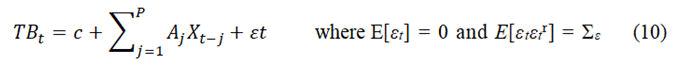
We start our specification with a reduced form trade balance equation described as follows, following Bahmani-Oskooee and Gelan. This is how the model can be displayed:

The explanatory variables in this model are the GDP (Y), and the real effective exchange rate (reer),T0 is trade openness, TOT is Terms of Trade and FDI is foreign direct investment. The trade balance is the dependent variable and εt, is stochastic error term we hold others factor constant even if we know that trade balance has numerous indicators, including trade liberalization, the elimination of anti-export bias, and import liberalization
The Gauss-Markov conditions for the linear regression model given by
Tb is trade balance as dependent variable, b is vector of the regression coefficients and εi, is disturbance term in matrix notation where
Gauss-Markov conditions should satisfy the following conditions
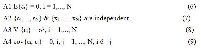
Spurious regressions which may arise as a result of carrying out regressions on time series data which are not stationary are suspected therefore OLS estimators is not relevant to our study, we use.
VAR model estimation approach
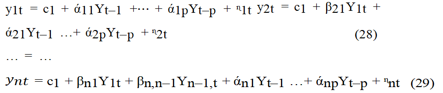
Since the contributions in Eichenbaum and Evans and Clarida and Gal, VAR methods have been largely used in the study of the current account and exchange rate. Following this approach, a five-variable structural VAR model of, real effective exchange rate, GDP per capita, trade openness, terms of trade, foreign direct investment. This specification incorporates the major insight of intertemporal models, namely that the current account is influenced by common rather than idiosyncratic (country-specific) shocks. This comes at the cost of identifying common ‘relative' shocks without distinguishing whether shocks originate in the national or the foreign economy. The long run, which is not consistent with models like the one presented here. The following is account the following reduced form VAR model.
Xt is the vector of n endogenous variables and c is an × 1 vector of intercepts. Aj is an n × n matrix comprising the AR-coefficients at lag j=1,..., P and εt is a vector of residuals with covariance matrix Σε=E[εtεtr], and Xt comprises the following n endogenous variables.

GDPt denotes the log level of the real gross domestic product, real effective exchange rate t, trade openness t, terms of trade t, foreign direct investment t [7].
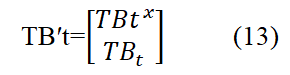
To capture spillover effects from foreign country shocks to domestic aggregates, we include the same set of variables for the foreign country in the VAR, which are denoted with an asterisk. Hence, we define:

The total set of variables included in the open-economy VAR framework are summarized as follows:
Statistic M(i) or the Akaike Information Criterion (AIC) have been used to identify the order, then estimate the specified model by using the least squares method (if there are statistically insignificant parameters, the model should be re-estimated by removing these parameters and finally use the Qk(m) statistic of the residuals to check the adequacy of a fitted model. Other characteristics of the residual series, such as conditional heteroscedasticity and outliers, can also be checked [8].
The time series Yt follows a VAR(p) model, if it satisfies

Where, Yt is a vector of the dependent variable Ф0 is a kdimensional vector and αt is a sequence of serially uncorrelated random vectors with mean zero and covariance matrix Σ. Covariance matrix Σ must be positive definite; otherwise, the dimension of Yt can be reduced. The error term, αt is a multivariate normal and Фj are k × k matrices. Using the back-shift operator B, the VAR(p) model can be written as:

Where, I will be the k × k identity matrix. In a compact form, it is as follows:
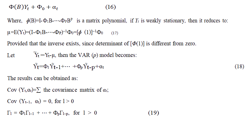
The equation (5) is a multivariate version of Yule Walker equation and it called the moment equation of a VAR(p) model. The concept of partial autocorrelation function of a is univariate series can be generalized to specify the order p of a vector series. Consider the following consecutive VAR models:
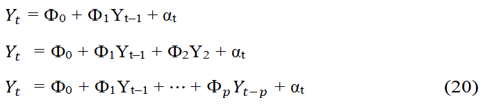
The Ordinary Least Squares (OLS) method is used for estimating parameters of these models. This is called the multivariate linear regression estimation in multivariate statistical analysis. For the equation in equation (5), let, Ф ̂j (i) be the OLS estimate of Фj and Ф ̂j (i) be the estimate of Ф0, where the superscript (i) is used to denote that the estimates are for a VAR(i) model. Then, the residual is:
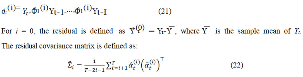
To specify the order p, the ith, and (i-1)th in equation (6) is to test a VAR(i) model versus a VAR(i-1) model and test the hypothesis H0:Фl=0 versus the alternative hypothesis Ha: Фl G 0 sequentially for i=1, 2, …, I. The test statistic is:
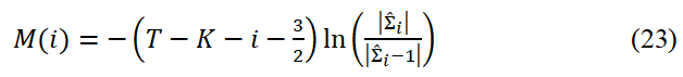
The distribution of M(i) is a chi-squared distribution with K2 degrees of freedom. Alternatively AIC can be used to select the order p. Assume that αt is multivariate normal and consider the ith equation, one can estimate the model by the Maximum Likelihood (ML) method. For AR models, the OLS estimates Ф0 and Фj are equivalent to the (conditional) ML estimates. However, there are differences between the estimates of Σ and the ML estimates of Σ.
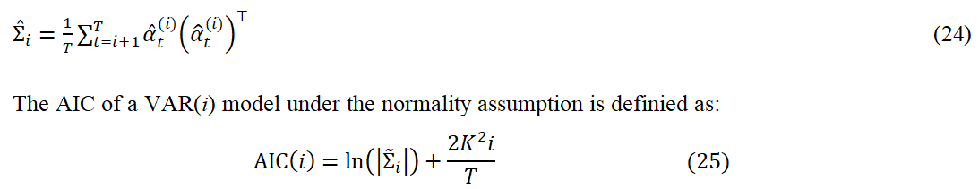
For a given vector time series, one selects the AR order p such that AIC(p)=min {1 ≤ i ≤ p, AIC(i)}, where p is positive integer.
Estimation and model checking both of the OLS method or the maximum likelihood method can be used to estimate parameters of VAR model, since the two methods are asymptotically equivalent. The estimates are asymptotically normal under some regularity conditions, after constructing the model, adequacy of the model should then be checked. The Qk(m) statistic can be applied to the residual series to check the assumption that there are no serial or cross-correlations in the residuals. For a fitted VAR(p) model, the Qk(m) statistic of the residuals is asymptotically a chi-square distribution with K2(m-g) degrees of freedom, where g is the number of estimated parameters in the AR coefficient matrices [9].
Structural analysis by impulse response functions
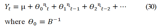
The general form VAR(p) model also has a wold representation as follows:

Where, θs are the n x n matrices. To interpret the (i,j)-th element θs, element of the matrix θs as the dynamic multiplier or impulse response:
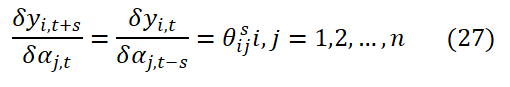
The condition for the variance of αt equal to Σ is a diagonal matrix. If Σ is diagonal, it shows that the elements of Σ and αt are uncorrelated. One way to make the errors uncorrelated is to estimate the triangular structural VAR(p) model:
The estimated covariance matrix of the error vector 5t is diagonal. The uncorrelated errors 5t are referred to as structural errors.
The Wold representation of Yt is based on the orthogonal errors 5t:
B is the lower triangular matrix of βij in equation (11). The diagonal elements of the B are 1. The impulse responses to the orthogonal shocks 5jt are:
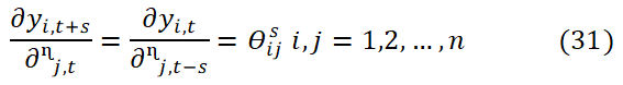
Whereϴij^s is the (i,j)th element of ϴs. The plot of ϴij^s against s is called the orthogonal impulse response function of yi with respect to ᶯj
Structural analysis by granger causality
In order to investigate the causal relationship among the variables of the system, the linear Granger causality tests should be applied by using the following strategy. Compare the unrestricted models:
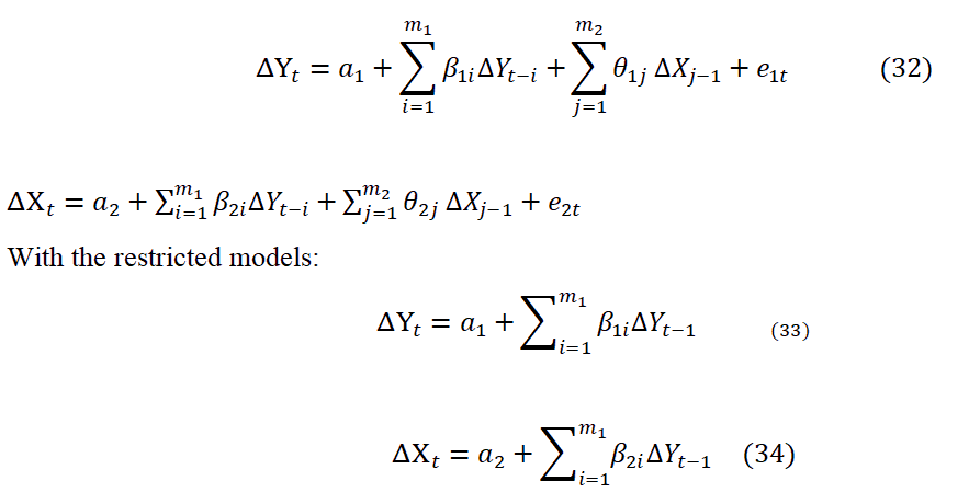
Where, ΔYt and ΔXt first order forward differences of the variables; α, β and ϴ are the parameters to be estimated; and e1 and e2 are standard random errors. The lag m are the optimal lag orders chosen by information criteria. The equations described above are convenient tools for analyzing linear causality relationship among the variables. If ϴ1 is statistically significant and ϴ2 is not, it can be said that changes in variable y Granger cause changes in variable x or vice versa. If both of them are statistically significant, there is a bivariate causal relationship among the variables; if both of them are statistically insignificant, neither the changes in variable y nor the changes in variable x have any effect over other variables [10].
Forecasting
If the fitted model is adequate, then it can be used to obtain forecasts. For forecasting, same techniques in the univariate analysis can be applied. To produce forecasts and standard deviations of the associated forecast, errors can be done as following. For a VAR(p) model, the 1-step ahead forecast at the time origin h is:
The associated forecast error is eh=ah+1. The covariance matrix of the forecast error is Σ. If Yt is weakly stationary, then the l-step ahead forecast Yh(l) converges to its mean vector μ as the forecast horizon increases.
Data
The paper uses BNR quarterly macroeconomic data over the period 2000 Q1 to 2020 Q4. The time series include trade balance as dependent variable and explanatory variables the real effective exchange rate (reer), GDP per capita (GDP_Ca) trade openness (TR), Terms of Trade (TOT) and Foreign Direct Investment (FDI) are converted into natural logarithms and come from the National Bank of Rwanda (NBR). The empirical study is based on quarterly data from 2000 Q1 to 2020 Q4 [11].
Variables definition
Trade Balance (TB) is the difference between a country's exports and imports in terms of money over a given time period is known as (Export-Import), sometimes known as net exports. The Real Effective Exchange Rate (REER) is the weighted average of a country's currency in respect to an index or basket of other important currencies. By comparing a country's currency's relative trade balance to those of every other country in the index, the weights are determined.
A country's Gross Domestic Product (GDP) per capita is calculated by dividing its GDP by its total population. Trade openness is the term used to describe how a country's economy is structured in relation to international trade. The size of an economy's recorded imports and exports serves as a proxy for the degree of openness.
The terms of trade are defined as the ratio of export prices to import prices and represent the relative cost of exports in relation to imports. It can be understood as the number of importable commodities an economy can buy for each unit of exportable goods. A foreign direct investment is a financial commitment made by a company with its headquarters in another nation to control a company in another country [12].
Results
Data descriptive as individual sample
The features of the variables seen in the short-, medium-, and longterm data from BNR are shown in Table 1 below. The variability in cross-sectional observations, which is supported by standard deviation statistics, is a characteristic shared by all the variables. Both the explanatory and the dependent variables are expressed in logarithmic form as follows: TB, Lnreer, LnGdp per capita, LnTo, LnTot and LnFdi, respectively (Table 1).
| CA | REER | GDP_PERCAPITA | TO | TOT | FDI | |
|---|---|---|---|---|---|---|
| Mean | -1.8711 | 82.12537 | 140.5376 | 34.96631 | 125.5582 | 34.37700 |
| Median | -1.7178 | 81.10288 | 152.7378 | 38.46799 | 135.7985 | 30.19320 |
| Maximum | -0.3623 | 98.40000 | 209.5449 | 59.40694 | 181.6496 | 105.9381 |
| Minimum | -3.9484 | 67.82000 | 60.21290 | 6.424578 | 70.98898 | 0.480466 |
| Std. dev. | 0.943754 | 7.244767 | 54.69618 | 17.16445 | 25.42189 | 29.48384 |
| Skewness | -0.3047 | 0.124433 | -0.32111 | -0.51663 | -0.66496 | 0.338412 |
| Kurtosis | 2.171058 | 2.137015 | 1.460049 | 1.738809 | 2.603907 | 1.800031 |
| Jarque-Bera | 3.704799 | 2.823370 | 9.743640 | 9.303780 | 6.739491 | 6.643051 |
| Probability | 0.156860 | 0.243732 | 0.007659 | 0.009544 | 0.034398 | 0.036098 |
| Sum | -157.172 | 6898.531 | 11805.16 | 2937.170 | 10546.89 | 2887.668 |
| Sum sq. dev. | 73.92571 | 4356.392 | 248308.8 | 24453.32 | 53640.63 | 72151.62 |
| Observations | 84 | 84 | 84 | 84 | 84 | 84 |
Table 1: Data descriptive as individual sample.
Unit root test (Test for stationarity)
The pre-test of the order of integration of the variables serves as the analysis's first step. In order to obtain the ordering of integration, we test for unit root to avoid this fruitless effort. Using the Augmented Dickey-Fuller (ADF) test, the test for stationarity is used to avoid spurious regressions which may arise as a result of carrying out regressions on time series data which are not stationary. Stationarity of time series was tested using the Augmented Dickey Fuller (ADF) tests. Professor Noman Arshed commented about OLS and cointegration as such: If all variables are I(0), no integration tests are required and OLS can be used. However, the regression of a nonstationary time series to another non non-stable time series may produce spurious to a non-sense regression (Table 2) [13].
| Variables | Level | First difference | Order of integration | ||
|---|---|---|---|---|---|
| Intercept | Trend | Intercept | Trend | ||
| TB | -4.49*** | 5.59*** | -10.54*** | -10.13*** | I(1) |
| LnGdp per capita | -2.28 | -2.89 | -7.86*** | -7.63*** | I(1) |
| Lnreer | -0.89 | -3.88** | -9.01* | -8.79* | I(1) |
| LnTo | -0.29 | -1.23 | -6.62* | -6.39* | I(1) |
| LnTot | -0.79 | -3.88** | -9.11* | -8.39* | I(1) |
| LnFdi | -0.16 | -1.23 | -5.62* | -6.38* | I(1) |
Note: *, **, ***:Denote rejection of null hypothesis at 10%, 5% and 1% significance level respectively
Table 2: Unit roots test for non-stationary data (Sample: 2000 Q1-2020 Q4).
Test for co-integration
Since all variables are non-stationary at levels, but became stationary at first difference. we performed a co-integration test using Johnsen cointegration tests based on unit root tests of regression residuals. Table 3 shows the results of the Johansen Cointegration test used to investigate whether there exists long-run relationship among the cointegrating variables which are are Trade balance as dependent variable and such as explanatory variables GDP (Y) and the real effective exchange rate (reer), trade openness (TR), Terms of Trade (TOT) and Foreign Direct Investment (FDI) (Tables 3 and 4) [14].
| Unrestricted cointegration rank test (Trace) | ||||
| Hypothesized No. of CE(s) |
Eigenvalue | Trace statistic |
0.05 Critical value |
Prob.** |
|---|---|---|---|---|
| None* | 0.451885 | 119.1654 | 95.75366 | 0.0005 |
| At most 1* | 0.275031 | 70.46255 | 69.81889 | 0.0444 |
| At most 2 | 0.238718 | 44.41077 | 47.85613 | 0.1016 |
| At most 3 | 0.163479 | 22.31793 | 29.79707 | 0.2812 |
| At most 4 | 0.066546 | 7.859179 | 15.49471 | 0.4806 |
| At most 5 | 0.027770 | 2.281203 | 3.841466 | 0.1309 |
Note: Trace test indicates 2 cointegrating eqn (s) at the 0.05 level Denotes rejection of the hypothesis at the 0.05 level**MacKinnon-Haug-Michelis (1999) p-values
Table 3: Test for co-integration.
| CA | GDP_CAPITA | REER | TO | TOT | FDI | |
|---|---|---|---|---|---|---|
| CA(-1) | 1.293997 | 0.930493 | 0.471692 | 0.229308 | 0.395743 | 0.620574 |
| (0.10621) | (0.78250) | (1.59639) | (2.32690) | (1.13239) | (7.60122) | |
| (12.1832) | ( 1.18912) | (0.29547) | (0.09855) | (0.34947) | (0.08164) | |
| CA(-2) | -0.48372 | -0.51688 | 0.007810 | 0.308642 | 0.017735 | 2.372929 |
| (0.10474) | (0.77166) | (1.57427) | (2.29466) | (1.11670) | (7.49589) | |
| (-4.61829) | (-0.66983) | (0.00496) | (0.13450) | (0.01588) | ( 0.31656) | |
| GDP_PERCAPITA(-1) | 0.012639 | 1.451722 | 0.042716 | 0.246905 | -0.07344 | -0.88576 |
| (0.01362) | (0.10032) | (0.20466) | (0.29831) | (0.14518) | (0.97449) | |
| (0.92825) | (14.4711) | (0.20871) | (0.82767) | (-0.50590) | (-0.90895) | |
| GDP_PERCAPITA(-2) | -0.01647 | -0.5129 | -0.00339 | -0.20975 | 0.117930 | 0.840846 |
| (0.01290) | (0.09507) | (0.19394) | (0.28269) | (0.13757) | (0.92346) | |
| (-1.27628) | (-5.39527) | (-0.01747) | (-0.74196) | (0.85722) | (0.91054) | |
| REER(-1) | -0.00322 | 0.084850 | 0.940626 | 0.027631 | -0.06701 | -0.55881 |
| (0.00906) | (0.06674) | (0.13616) | (0.19846) | (0.09658) | (0.64831) | |
| (-0.35577) | (1.27135) | (6.90837) | (0.13923) | (-0.69376) | (-0.86194) | |
| REER(-2) | 0.000430 | -0.11666 | -0.07181 | -0.09099 | 0.050547 | 0.189657 |
| (0.00867) | (0.06387) | (0.13029) | (0.18992) | (0.09242) | (0.62040) | |
| (0.04957) | (-1.82657) | (-0.55114) | (-0.47912) | (0.54691) | (0.30570) | |
| TO(-1) | 0.003818 | 0.045626 | 0.008665 | 0.564563 | 0.046584 | 0.941083 |
| (0.00596) | (0.04394) | (0.08965) | (0.13067) | (0.06359) | (0.42685) | |
| ( 0.64015) | (1.03832) | (0.09666) | (4.32058) | (0.73257) | (2.20471) | |
| TO(-2) | -0.001 | 0.106809 | -0.08214 | 0.086334 | 0.056262 | 0.011346 |
| (0.00626) | (0.04610) | (0.09405) | (0.13708) | (0.06671) | (0.44780) | |
| (-0.15996) | (2.31699) | (-0.87336) | (0.62981) | (0.84338) | (0.02534) | |
| TOT(-1) | 0.012921 | -0.00495 | 0.240972 | 0.106129 | 1.812866 | -0.55194 |
| (0.00641) | (0.04721) | (0.09631) | (0.14038) | (0.06832) | (0.45858) | |
| (2.01641) | (-0.10474) | (2.50204) | (0.75600) | (26.5360) | (-1.20358) | |
| TOT(-2) | -0.01213 | 0.033739 | -0.24257 | -0.03985 | -0.8985 | 0.459439 |
| (0.00672) | (0.04948) | (0.10095) | (0.14714) | (0.07161) | (0.48066) | |
| (-1.80554) | (0.68186) | (-2.40291) | (-0.27084) | (-12.5478) | ( 0.95585) | |
| FDI(-1) | -0.00084 | 0.017722 | -0.00401 | 0.004400 | -0.03381 | 0.471624 |
| (0.00169) | (0.01247) | (0.02544) | (0.03708) | (0.01805) | (0.12113) | |
| (-0.49369) | (1.42123) | (-0.15744) | (0.11866) | (-1.87361) | (3.89355) | |
| FDI(-2) | 0.000888 | -0.00664 | 0.010489 | 0.084534 | -0.03767 | 0.163607 |
| (0.00172) | (0.01268) | (0.02586) | (0.03770) | (0.01835) | (0.12316) | |
| (0.51586) | (-0.52406) | (0.40553) | (2.24225) | (-2.05307) | (1.32846) | |
| C | 0.163110 | 3.482958 | 8.391647 | 1.932112 | 5.858460 | 34.70804 |
| (0.27654) | (2.03742) | (4.15655) | (6.05860) | (2.94844) | (19.7914) | |
| (0.58981) | (1.70950) | (2.01890) | (0.31890) | (1.98697) | (1.75369) | |
| R-squared | 0.969311 | 0.999489 | 0.870418 | 0.952919 | 0.995137 | 0.836526 |
| Adj. R-squared | 0.963974 | 0.999400 | 0.847882 | 0.944731 | 0.994291 | 0.808095 |
| Sum sq. resids | 2.235907 | 121.3627 | 505.1171 | 1073.172 | 254.1609 | 11451.97 |
| S.E. equation | 0.180012 | 1.326228 | 2.705649 | 3.943757 | 1.919242 | 12.88296 |
| F-statistic | 181.6157 | 11246.53 | 38.62358 | 116.3789 | 1176.579 | 29.42373 |
| Log likelihood | 31.33201 | -132.428 | -190.894 | -221.791 | -162.734 | -318.86 |
| Akaike AIC | -0.44712 | 3.547015 | 4.973021 | 5.726605 | 4.286199 | 8.094148 |
| Schwarz SC | -0.06557 | 3.928568 | 5.354574 | 6.108158 | 4.667752 | 8.475701 |
| Mean dependent | -1.8887 | 142.3093 | 81.76209 | 35.66043 | 126.1909 | 35.15736 |
| S.D. dependent | 0.948409 | 54.14852 | 6.937162 | 16.77519 | 25.40078 | 29.40850 |
| Determinant resid covariance (dof adj.) | 2674.530 | |||||
| Determinant resid covariance | 949.4212 | |||||
| Log likelihood | -979.208 | |||||
| Akaike information criterion | 25.78555 | |||||
| Schwarz criterion | 28.07487 | |||||
Table 4: VAR model.
Table 4 shows the computed VAR coefficients results show that the real effective exchange rate has no effect on trade balance in the short run but improves trade balance in the long run. Because there are so many criteria, presenting them all is time-consuming. Furthermore, they are underestimated: With the exception of the first personal lag, they are all minor. As a result, it is common to provide functions of the VAR coefficients discussed above that condense information, have some economic relevance and are, ideally, more properly assessed. Among the numerous functions available, three are commonly used: Impulse responses, variance, and historical decompositions. The impulse responses trace out the system's moving average, describing how it responds to a shock; the variance decomposition measures the contribution to the variability of the real effective exchange rate; and the historical decomposition describes the contribution of Rwanda's current account shock to deviations from its baseline forecasted path from 2000 Q1 to 2020 Q4. Since we don’t use ARDL in our study, we fail to estimate short run speed of adjustment coefficient and Long run speed of adjustment coefficient.
Granger causality tests
Granger causality test is use a statistical test to see if one-time series may predict another. The hypothesis would be rejected at that level if the probability value was less than 0.05. In our case we fail to reject HO which means that the long-run coefficient indicated that a 1 percent real effective exchange rate would lead to improvement in Rwanda's trade balance (Table 5) [15].
| Null hypothesis | Obs. | F-statistic | Prob. |
|---|---|---|---|
| REER does not granger cause CA | 82 | 0.30880 | 0.7352 |
| CA does not granger cause REER | - | 0.78386 | 0.4602 |
Table 5: Granger causality tests.
Impulsive response for rwanda
Base on VAR impulsive response in our variables which are Trade balance as dependent variable and explanatory variables the real effective exchange rate (reer), GDP per capita (GDP Ca), trade openness (TR), Terms of Trade (TOT) and Foreign Direct Investment (FDI). VAR impulse responses react to the identified spillover effect on demand and supply shocks and evidence for spillover effects from Rwanda demand shocks and Central interest rate policy shocks as follows (Figure 5).

Figure 5: Response to cholesky one s.d.innovation s ± 2 S.E.
• VAR impulsive response shows that in the foreign exchange
markets, a rising current account deficit in Rwanda causes a rise in
the supply of Rwandan francs. There will be an outward movement
in supply on the market for Rwandan francs as a result. Ceteris paribus, this could result in a decline in the Rwandan franc's
external value [16].
• VAR impulse response demonstrates that in the short-run, there is a
poor correlation between changes in the current account deficit and
per-capita GDP.
• VAR Impulse response show the favorable impact of trade openness
on the current account suggests that an economy can improve the
current account more quickly with fewer trade barriers and greater
exposure.
• VAR Impulse response indicate When the value of imports rises
faster than the value of exports, the trade balance in Rwanda
deteriorates, which causes shocks to the terms of trade in Rwanda.
• VAR Impulse response show that Increased Foreign Direct
Investment (FDI) into Rwanda could lead to increased economic
investment of Rwanda, which would improve Rwanda current
account. However, increase the volume of foreign direct investment
in Rwanda also increases the sizes of import and profit repatriation
[17].
Conclusion
The paper uses quarterly macroeconomic data from BNR for the period 2000 Q1 to 2020 Q4. The time series include trade balance as dependent variable and explanatory variables, real effective exchange rate, GDP per capita, trade openness, trade conditions and foreign direct investment. Several studies have since tried to prove this connection. According to some theories, a nation's trade balance will deteriorate if its currency depreciates or depreciates before it reverses in the long term. This phenomenon is known in the literature as the Jcurve effect. These studies started from the assumption that the trade balance and exchange rate movements are linearly related. Our research shows that Rwanda's export growth has typically lagged its import growth, widening the trade deficit to the point where it could potentially trigger a financial crisis. The data were transformed to the natural logarithm. According to our findings, all variables at I(1) are stationary, which means that there is a long-run relationship between the cointegrating variables. The results of the Granger causality test show that the long-run coefficient indicated that a 1 percent real effective exchange rate would result in an improvement in Rwanda's trade balance. AR impulse responses respond to the identified spillover effect on demand and supply shocks and evidence of spillover effects from demand shocks in Rwanda and central interest rate policy shocks.
This study recommends to policymakers that a devaluation of the Rwandan franc improves the trade balance in the long term, all things being equal, and an increase in Foreign Direct Investment (FDI) in Rwanda could lead to increased Rwandan economic investment, which would improve Rwanda's current account balance. However, increasing the volume of foreign direct investment in Rwanda also increases imports and the repatriation of profits. Finally, this study also recommends additional research using more reliable methods to learn more about how exchange rates affect changes in Rwanda's trade balance.
Declaration of Competing Interests
None.
Acknowledgement
We acknowledge the national bank of Rwanda's data providers.
References
- Arize A, Malindretos CJ, Igwe EU (2017) Do exchange rate changes improve the trade balance: An asymmetric nonlinear cointegration approach. Int Rev Eco Fin 49: 313-326.
- Bahmani-Oskooee M, Gelan A (2019) the South Africa-U.S. trade and the real exchange rate: Asymmetric evidence from 25 industries. South Afr J Econ 12: 1-17.
- Bahmani-Oskooee M, Kovyryalova M (2008) Impact of exchange rate uncertainty on trade flows evidence from commodity trade between the United States and the United Kingdom. World Econ 31: 1097-1128.
- Bahmani-Oskooee M, Fariditavana H (2016) Nonlinear ARDL approach and the j-curve phenomenon. Open Econ Rev 27: 51-70.
- Bahmani-Oskooee M (1985) Devaluation and the J-curve: Some evidence from LDCs. Rev Econ Statc 67: 500-504.
- Banerjee A, Dolado J, Mestre R (1998) Error-correction mechanism tests in a single equation framework. J Time Seri Analy 19: 267-285.
- Bickerdike CF (1920) The instability of foreign exchanges. Econ J 30: 118-122.
- Bleaney M, Tian M (2014) Exchange rates and trade balance adjustment: A multi-country empirical analysis. Open Econ Rev 25: 655-675.
- Breusch TS (1978) Testing for autocorrelation in dynamic linear models. Aus Econ Paper 17: 334-355.
- Cardarelli R, Rebucci A (2007) Exchange rates and the adjustment of external imbalances. Chap World Econ Outlook 81-120.
- Chiloane L, Pretorius M, Botha I (2014) The relationship between the exchange rate and the trade balance in South Africa. J Econ Fin Sci 7: 299-314.
- Dornbusch R (1971) Notes on growth and the balance of payments. Can J Econ 7:389-395.
- Durmaz N (2015) Industry level J-Curve in Turkey. J Eco Stud 42: 689-706.
- Frankel JA (1971) A theory of money, trade, and balance of payments in a model of accumulation. J Int Econ 12: 158-187.
- Ghatak S, Siddiki J (2001) The use of the ARDL approach in estimating virtual exchange rates in India. J App Statist 11: 573-583.
- Guechari Y (2012) An empirical study on the effects of real effective exchange rate on Algeria’s trade balance. Int J Fin Res 3: 102-115.
- Jimoh A (2004) The monetary approach to exchange rate determination: Evidence from Nigeria. J Eco Cooper 25: 109-130.