Research Article, J Mar Biol Oceanogr Vol: 8 Issue: 1
Hydro-Climatic Variations Analysis with Remote Sensing Data on Sri Lankan Ocean Water
Thushani Suleka Madhubhashini Elepathage1,2* and Danling Tang1,2
1South China Sea Institute of Oceanology, Chinese Academy of Sciences, Guangzhou, China
2University of Chinese Academy of Sciences, Beijing 100049, China
*Corresponding Author : Thushani Suleka Madhubhashini Elepathage
South China Sea Institute of Oceanology, Chinese Academy of Sciences, Guangzhou, China
Tel: 15626139343
E-mail: thushani@scsio.ac.cn
Received: May 03, 2019 Accepted: June 18, 2019 Published: June 26, 2019
Citation: Madhubhashini Elepathage TS, Tang D (2019) Hydro-Climatic Variations Analysis with Remote Sensing Data on Sri Lankan Ocean Waters. J Mar Biol Oceanogr 8:1.
Abstract
This study modeled the future trends of physical, chemical, and biological changes in the Sri Lankan ocean region after examining their trends, similarities, and differences. Many types of satellite data were used to extract oceanographic and atmosphere variables. The atmospheric and hydrologic interactions were identified and the time series expert modeler criteria were used to predict the future trend of each analysed variable. Principle component analysis (PCA) was used to reveal patterns in the overall variability of ocean and atmosphere variables. In order to identify the relationship between the atmospheric and other affecting variables with the oceanographic variables, the canonical correlation analysis was conducted. Time series plots within the past 30 years clearly show Sea surface temperature, sea salt surface mass concentration, specific humidity, Carbon monoxide (CO) emission, Iron concentration, Ultra-violet (UV) aerosol index have clear increasing trends. Sulphate (SO4) extinction, SO4 column mass density, Sulphide (SO2) surface mass concentration, methane total column concentration, Carbon dioxide (CO2) emission have shown extreme increments within the past 15 years. According to the time series expert modeler criteria predictions, carbon dioxide (0.0058-mole fraction month-1), organic carbon surface mass concentration (1×10-13 kgm-3 month-1) has drastic increments in the future.
Keywords: Atmosphere; Ocean; Canonical correlation analysis; Principal component analysis; Remote sensing
Introduction
The effects of climate change are accelerating on marine ecosystems. The increased heating at a value of about 3 Wm-2 in the lower atmosphere or earth’s surface resulting from the ‘greenhouse’ effect caused by increasing atmospheric CO2, methane and other greenhouse gasses have already made direct physical consequences on the marine environment and marine species. Climate change is one of the factors, which makes the adverse effects such as loss of aquatic habitat, pollution, fish deaths, disturbances and the introduction of fish species that may exotic and invasive to the new environments [1]. The study of the changing ocean encompasses several features as well as the interaction of the ocean with land, the cryosphere, and the atmosphere [2].
Except in a band centered at about 12°S (South Equatorial Current), the upper area of the Indian Ocean has been warming all around continuously [1]. The upper 100 m of tropical and Eastern subtropical Indian Ocean (in around north of 10°S), is getting warmed drastically. A significant increment of warming in the sea surface can be seen from 1990-1999 [3]. Over the past decades, climate change in the tropical western Pacific has led to surface warming in the South China Sea (SCS), which makes profound impacts on marine ecosystems and coastal communities [4]. Therefore, it is imperative to understand the environmental changes in the ocean areas in order to provide recommendations to mitigate future climate-related problems.
Climate change has a potential impact on the food production system and thus, food security in the Pacific Island countries (PICs), including Solomon Islands [5]. The most immediate impacts of climate change include further reductions in fisheries and aquaculture production due to rising sea temperatures, ocean acidification, and sea level. Habitat and coastal barriers are destroyed and fish populations face serious problems. Due to population growth, urban development and the loss of fish habitats, coastal fishing activities are an integral part of the livelihood economy in the Pacific Island countries and overfishing may occur. In some cases, some fish can be favored by climate change, but these benefits can be compensated if there are extreme conditions of humidity or dry conditions [5].
Sri Lanka is also experiencing several difficulties due to climate change. The main effects that can be seen in Sri Lankan region are increasing in temperature, more frequent droughts, erratic rainfalls, and rise in sea level [6]. Especially the coastal economy is affected by the sea level rise (SLR) in Sri Lanka which is 0.3 m by 2010. The atmospheric and water changes have affected several other sectors such as agriculture, forest, biodiversity, health, energy, human settlements, fisheries, and tourism, etc.
Since the adaptation and mitigation methods that are selected to overcome climate change impacts directly affect to the future sustainability of many economic sectors, these strategies should be autonomous and planned. The intentional adaptation to avoid unhealthy adaptation needs to consider which species, community or ecosystem is most vulnerable to the impacts of climate change; the possibility that climate-friendly changes affect the industries involved; and what planned adaptation measures can be implemented to effectively cope with future changes [7]. To select the best mitigation measures it is important to understand the changes happening in each region separately. Hence, this study investigated the physical, chemical, and biological changes caused by climate changes in the Sri Lankan ocean areas and modeled the future trends in order to take the adaptation measures in response to climate change.
Study Areas and Methods
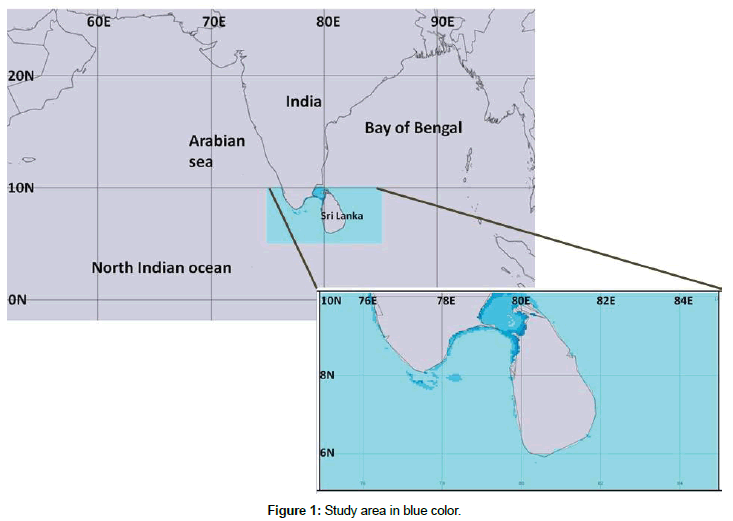
The area which is mainly covering the Sri Lankan Exclusive Economic Zone was selected. The Figure 1 indicates the study area with coordinates.
Atmospheric infrared sounder (AIRS) data were used to obtain the relative humidity. Modern-Era Retrospective analysis for Research and Applications (MERRA)-2 data were used to extract the Vertical pressure velocity, Wind Speed at 50 m above displacement height, surface wind stress, anomaly of aerosol optical depth 550 nm, sensible heat flux from turbulence, sea salt surface mass concentration, SO4 surface mass concentration, SO2 surface mass concentration, open water net downward long wave flux, black carbon column mass density, SO4 column mass density, total ozone analysis tendency, ozone mass mixing ratio, organic carbon column mass density, organic carbon surface mass concentration, upwelling long wave flux, surface incoming shortwave flux under clear sky, open water latent energy flux, evaporation from turbulence, surface absorbed long wave radiation, CO emission and black carbon surface mass concentration. MERRA 3D IAU State, meteorology monthly means were used for specific humidity and air temperature. Sea-viewing Wide Field-ofview Sensor (SeaWiFS) was used to get aerosol optical depth 550 nm in ocean-only), Chl-a concentration. Moderate Resolution Imaging Spectroradiometer (MODIS) Level 3 data was used for scattering angle and Chl-a. Global Land Data Assimilation System (GLDAS) Noah Land Surface model was used to storm-surface runoff, canopy water evaporation. Tropical Rainfall Measuring Mission (TRMM) data were used for latent heating and precipitation. NASA Ocean Biogeochemical Model (NOBM) was used to obtain NASA ocean biogeochemical model assimilating ESRID data were used to get nitrate and iron. Ocean color and temperature scanner (OCTS) was used to analyze the diffuse attenuation coefficient for downwelling irradiance at 490 nm. Atmospheric infrared sounder (AIRS)/Aqua data were used to extract carbon dioxide, mole fraction in the free troposphere, ethane total column. Test Operations Management System (TOMS) Nimbus-7 total ozone aerosol index UV-reflectivity UV-B erythemal irradiances were used to obtain UV aerosol index. Not only the oceanographic data but the variables that effect on atmosphere also were analyzed to identify the atmospheric and hydrologic interactions. The time series expert modeler criteria were used to predict the future trend of each analyzed variable. The Principal Component Analysis (PCA) was used to identify the components of the dataset that maximizes variance; making standard linear models potentially more powerful were identified [8]. In order to identify the relationship between the atmospheric and other affecting variables with the oceanographic variables, the canonical correlation analysis was conducted [9,10].
Results
The physical, chemical, and biological changes caused by climate changes in the Sri Lankan ocean areas
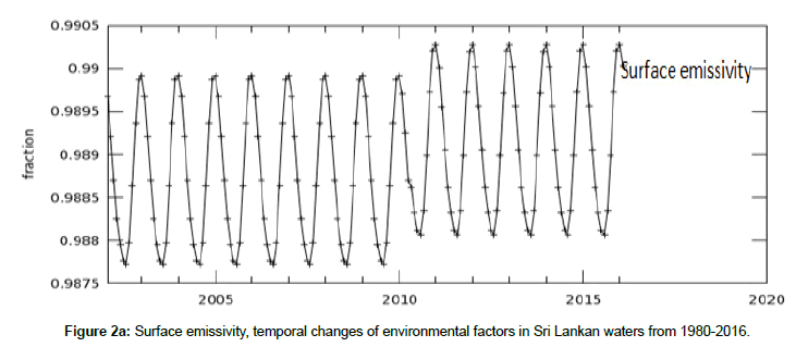
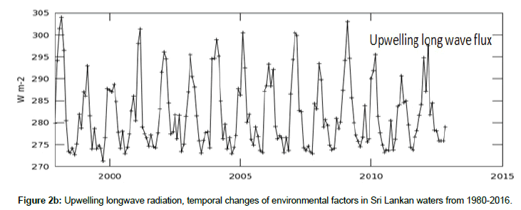
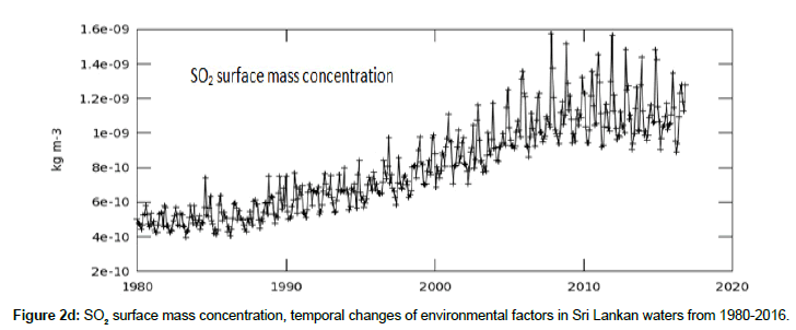
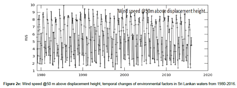
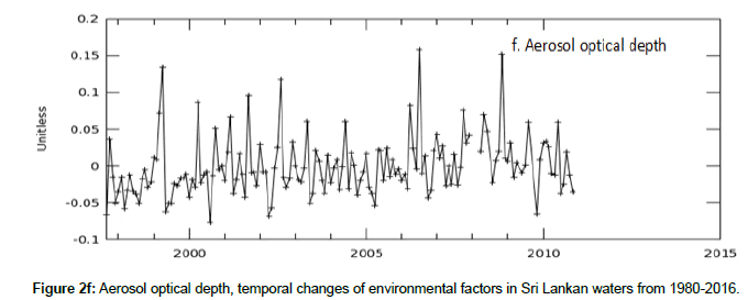
Identification of the increment and decrease can be basically done by analyzing the satellite images over the study period and plotting the extracted data. The monthly mean changes over the study period are shown in Figures 2a-2e below. According to the plots and the calculations, carbon dioxide (0.7997 ppm per month), surface absorbed long wave radiation (0.2502 Wm-2 per month), surface incoming short wave flux (0.1429 Wm-2 per month), upwelling long wave flux (0.1425 Wm-2 per month), scattering angle (0.0573 per month), sea surface temperature (0.0197°C per month), open water latent energy flux (0.0099 Wm-2 per month), total water vapour (0.0096 kgm-2 per month), surface emissivity (0.0007 per month), sulfur dioxide surface mass concentration (0.0137 kgm-3 per month), sulphate surface mass concentration (0.5188 kgm-3 per month), nitrate concentration (0.0020 micromolesL-1 per month) have considerably increasing trends. However, ozone tendency, sensible heat flux from turbulence changes have been decreased after about 2004 while black carbon surface mass concentration changes have been increased after about 2004. Wind speed (-0.0002 ms-1 month-1), sensible heat (-0.1307), the anomaly of aerosols (-0.1308) also have decreasing trends.
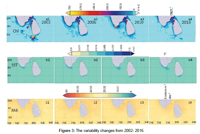
Figure 3 consists of 3 example maps of Chl-a, SST and photosynthetically available radiation (PAR) to show the changes of these variables from the beginning of the study period to end. Figures 3a1-3a4 prove there is a decrease of Chl-a with the time and Figures 3b1-3b4 & 3c1-3c4 show a considerable increase in SST and PAR.
The future changes in the variables
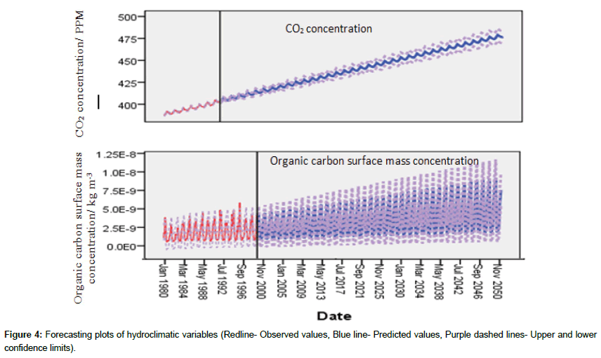
With time series analysis the future trends of each variable were predicted until 2050. Statistically significant (with 5% significance level) predicted variables were selected which had been correctly specified. The time series expert modeler criteria is a statistical option which automatically identifies and estimates the best-fitting Auto-Regressive Integrated Moving Average (ARIMA) or exponential smoothing model for one or more dependent variable series [11]. Univariate (single vector) ARIMA is a forecasting technique that projects future values of a series based entirely on its own inertia. Its main application is in the area of short term forecasting requiring at least 40 historical data points. The simplest of the exponentially smoothing methods is naturally called “simple exponential smoothing” (SES). This method is suitable for forecasting data with no trend or seasonal pattern. In exponential smoothing (as opposed to in moving averages smoothing) older data is given progressively-less relative weight (importance) whereas newer data is given progressively-greater weight. Also called averaging, it is employed in making short-term forecasts. According to the time series expert modeler criteria predictions, carbon dioxide, organic carbon has drastic increments in the future (Figure 4).
According to the forecasting plots in Figure 4 the CO2 concentration shows a similar increasing rate in the future as it has shown until 2000. However, if the CO2 concentration will increase at the same rate it can reach even up to 475 PPM by 2050. Organic carbon surface mass concentration has high inter-annual variability. Hence the forecasting line also shows high variability and high upper confidence limits and lower confidence limits. However, the trend is similar to the past trend that can be seen up to 2000.
The following plots which indicate the seasonal variations of the variables give an idea of how the seasonal changes happen within the study period and which seasons have a higher increase or decrease of the relevant variable.
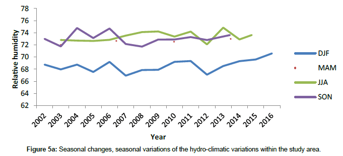
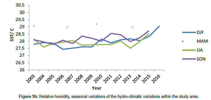
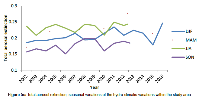
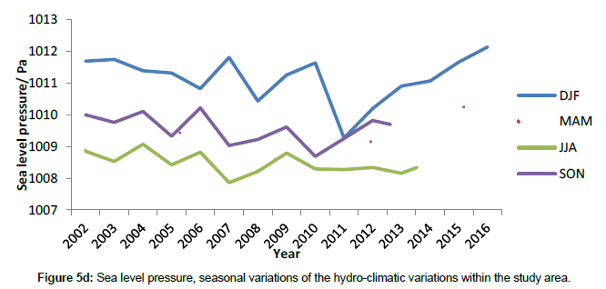
When the time series plots were analyzed from 2002-2016, sea surface temperature, relative humidity, sea level pressure, and total aerosol index have clear increasing trends other than their seasonal changes (Figures 5a-5d).
SO4 extinction, SO4 column mass density, SO2 surface mass concentration, methane total column concentration, CO2 emission show extreme increments. However, ozone tendency, sensible heat flux from turbulence changes have been decreased after about 2004 while black carbon surface mass concentration changes have been increased after about 2004.
According to the seasonal variations of the variables, sea salt scattering Aerosol optical depth is higher in June, July and August months than other months. It has changed from around 0.05 to 0.09. Sea salt extinction is also highest in June, July and August months. The sea level pressure and time-averaged surface pressure is lower than the other months in previously stated months. The sea level pressure and time-averaged surface pressure is higher in December, January and February than other months.
The highest mean temperatures at 2 m and 10 m displacement heights and the specific humidity at 2 m and 10 m displacement height can be seen mostly in March, April and May months. All of the above variables are lowest in December, January, and February months. However, relative humidity is highest in June, July, and August months through the lowest months are similar to temperature and specific humidity.
Black carbon column mass density, black carbon surface mass concentration, methane total column concentration, and black carbon scattering have an increasing trend and it is lowest in June, July and August months. Mostly it is highest in December, January, and February months. The SO4 extinction, aerosol optical depth, total optical depth, and total aerosol extinction have a huge increment of 1982 and 1992.
CO column burden, CO chemical loss has huge increments in 1997 especially in September, October, and November months. CO chemical production is higher in March, April and May months and usually lowest in December, January, and February. CO2 mole fraction has an increasing trend and the highest values are in June, July, and August months. The lowest can be seen in December, January, and February. In September, October and November plant canopy surface water is high. Mean Diffuse attenuation coefficient and Chl-a concentration is higher in June, July and August months and lowest in March, April and May months. The cloud fraction for radiation is highest in December, January, and February months. Mass fraction of cloud is highest in December, January, and February while the lowest can be seen in June, July, and August. Dust dry deposition and dust extinction have drastic increments in March-August from 2000. Surface emissivity is highest in December, January, and February months and lowest in June, July, and August. Until 1995, CO extinction is high during December- May months. However, the CO extinction shows a decreasing trend after 1995 in the above months and the mean CO during June- August has increased after 1995. Total latent energy is comparatively high in June, July and August months while the highest sea surface temperature, photosynthetically available radiation and mean sensible heat flux are available in March, April, and May. Surface absorbed long wave radiation is lowest in December, January, and February months. Ground heating is highest in March, April, and May months. Evaporation from turbulence can be highest in June, July, and August and open water upward sensible heat flux is lowest the same months. The standard deviation of aerosol optical depth is highest in June, July, and August months. Surface skin temperature is highest in March, April, and May and it is lowest in December, January, and February. Ertel's potential vorticity is highest in June, July and August months and lowest in March, April, and May. Eastward surface wind stresses, as well as Northward surface wind stress, are highest in June, July, and August months while lowest in December, January and February months. Surface wind speed and wind speed at 10 m above displacement height are highest in June, July, and August and they are lowest in March, April, and May. Vertical pressure velocity is highest in December, January, and February. Dust extinction and dust scattering are highest in June, July, and August.
The relationship between hydro-climate variables
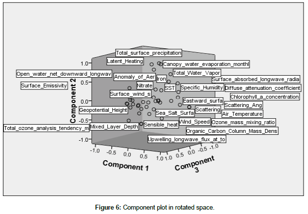
According to the PCA analysis scree plot, the first three principal components are more important. Projection of the variables on the factor plane revealed that the 1st and the 2nd axes of the PCs explained 30.55% and 12.68% of the total variance (Figure 6). The 3rd component explained only 6.02%. The principal component analysis is a linear transformation that chooses a variable system for the data set such that the greatest variance of the data set comes to lie on the first axis (or the principal component), the second greatest variance on the second axis, and the third greatest variance on the third [12].
The principal components are the eigenvectors of the covariance matrix of the original dataset. Because the covariance matrix is symmetric, the eigenvectors are orthogonal. When analyzed with Oblimin and Kaiser normalization the first component was described by open water latent energy flux, mean scattering angle, surface incoming short wave flux, evaporation from turbulence, sensible heat, surface winds, chll-a concentration, nitrate concentration, air temperature, leaf area index, CO2 concentration, sea salt concentration, eastward surface wind speed, sea surface temperature, surface emissivity, diffuse attenuation coefficient, carbon dioxide mass density, SO2 surface mass density, geo-potential height, ozone mass mixing ratio, wind speed, mixed layer depth, vertical pressure, specific humidity, SO4 surface mass density, surface absorbed long wave radiation, CO emission and black carbon surface mass concentration.
Principal component 2 was described by organic carbon surface mass concentration, black carbon column mass density, total ozone analysis tendency, storm surface, upwelling long wave flux at top of atmosphere, latent heating, organic carbon column mass density, open water net downward long wave, total water vapour total precipitation, total surface precipitation, black carbon surface mass concentration, canopy water evaporation, iron concentration, specific humidity, SO4 surface mass density, surface absorbed long wave radiation, CO emission and ozone mass mixing ratio.
Principal component 3 was described by leaf area index, eastward surface wind speed, sea surface temperature, surface emissivity, diffuse attenuation coefficient, carbon dioxide concentration, SO2 surface mass density, mixed layer depth, vertical pressure, specific humidity, SO4 surface mass density, surface absorbed long wave radiation, storm surface, upwelling long wave flux at top of atmosphere, open water net downward long wave, total water vapour total precipitation, total surface precipitation, black carbon surface mass concentration, anomaly of aerosols, canopy water evaporation and iron concentration.
When the components were plotted according to Oblimin with Kaizer normalization rotation method, the plot shows how closely related the items are to each other and to the three components. The plot of component loadings shows that chlorophyll-a concentration, open water latent, energy flux, evaporation from turbulence, nitrate concentration, evaporation from turbulence, surface winds, sensible heat, diffuse attenuation coefficient, sea salt concentration, wind speed all load highly and positively on the first component, storm surface latent heating on second component and anomaly of aerosols on third component.
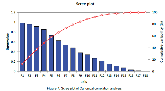
Canonical Correlation analysis is the analysis of multiple-X multiple-Y correlation. The Canonical Correlation Coefficient measures the strength of association between two Canonical Variates. The general fit of the model reporting Pillai's, Helling's, Wilk's and Roy's multivariate criteria are indicated in the table above. The commonly used test is Wilk's lambda, and we found that all of the tests such as Pillais, Hotellings, Wilks, Roys tests are significant with p<0.05. Eigen values and canonical correlations report the first canonical correlation coefficients and the eigen values of the canonical roots. The first canonical correlation coefficient is 0.99854 with an explained variance of the correlation of 64.66% and an eigen value of 341.29. Thus indicating that our hypothesis is correct- the atmospheric variables and the oceanic variables are positively correlated. The above table shows the significance of each of the roots. We found that of the twelve possible roots only the first five roots are significant with p<0.05. Since our model contains the 20 oceanic variables and 12 influencing variables, the canonical correlation analysis extracts 12 canonical roots or dimensions. The first five significance tests of all 12 canonical roots are (f=7.89, f=5.31103, f=3.64293, f=2.69325, f=1.87633 and p<0.05). Standardized canonical coefficients obtained for covariates show the standardized canonical loadings for each of the dependent variables. The variables with the highest canonical loadings are the most strongly related to the latent dependent variables- so in this case, “surface winds” has the strongest association with the underlying construct, and “greenness factor” the lowest association with it according to the first root number. Sequentially, organic carbon column mass density according to the second root, evaporation from the turbulence according to the third root, Black carbon column mass density according to the fourth root, surface incoming short wave flux according to the fifth root number as the strongest association with the underlying construct. Table 1 (canonical correlation matrix) show clearly the correlated and anti-correlated variables which have been further discussed. The following Figure 7 (scree plot) indicates how the Eigenvalues are distributed in Canonical correlation analysis and the first 5 canonical roots are significant.
| No | Variables | 1 | 2 | 3 | 4 | 5 | 6 | 7 | 8 | 9 | 10 | 11 | 12 | 13 | 14 | 15 | 16 | 17 | 18 | 19 | 20 | 21 | 22 | 23 | 24 | 25 | 26 | 27 | 28 | 29 | 30 | 31 | 32 | 33 | 34 | 35 | 36 | 37 | 38 |
|---|---|---|---|---|---|---|---|---|---|---|---|---|---|---|---|---|---|---|---|---|---|---|---|---|---|---|---|---|---|---|---|---|---|---|---|---|---|---|---|
| 1 | Vertical pressure | 1.0 | -0.2 | -0.2 | -0.6 | -0.1 | 0.0 | 0.3 | -0.1 | 0.2 | 0.4 | 0.4 | -0.6 | -0.6 | 0.6 | -0.3 | -0.2 | 0.5 | -0.5 | -0.4 | -0.5 | -0.3 | -0.1 | -0.2 | -0.3 | -0.5 | 0.4 | 0.2 | -0.2 | -0.6 | -0.1 | 0.3 | -0.1 | 0.1 | 0.1 | 0.1 | -0.1 | -0.1 | -0.1 |
| 2 | Wind speed | -0.2 | 1.0 | 0.9 | 0.8 | 0.0 | 0.0 | -0.2 | -0.2 | -0.5 | -0.5 | -0.4 | 0.1 | 0.3 | -0.4 | 0.0 | -0.2 | -0.5 | 0.4 | 0.1 | 0.4 | 0.0 | 0.0 | -0.1 | 0.8 | -0.1 | -0.4 | 0.0 | 0.1 | 0.6 | 0.2 | 0.2 | 0.0 | 0.0 | 0.8 | 0.8 | 0.8 | 0.2 | 0.3 |
| 3 | Surface winds | -0.2 | 0.9 | 1.0 | 0.7 | 0.0 | 0.0 | -0.2 | -0.2 | -0.5 | -0.5 | -0.5 | 0.1 | 0.3 | -0.4 | 0.1 | -0.2 | -0.4 | 0.4 | 0.1 | 0.5 | 0.2 | 0.0 | -0.2 | 0.9 | -0.1 | -0.3 | 0.1 | 0.2 | 0.6 | 0.2 | 0.2 | 0.0 | 0.1 | 0.8 | 0.8 | 0.8 | 0.3 | 0.3 |
| 4 | Eastward surface winds | -0.6 | 0.8 | 0.7 | 1.0 | 0.1 | -0.1 | -0.5 | 0.0 | -0.5 | -0.6 | -0.6 | 0.6 | 0.7 | -0.8 | 0.2 | 0.0 | -0.6 | 0.7 | 0.5 | 0.7 | 0.2 | 0.1 | 0.1 | 0.7 | 0.3 | -0.5 | -0.1 | 0.2 | 0.8 | 0.3 | -0.1 | 0.1 | 0.1 | 0.4 | 0.4 | 0.5 | 0.3 | 0.3 |
| 5 | Anomaly of Aerosol | -0.1 | 0.0 | 0.0 | 0.1 | 1.0 | 0.0 | 0.0 | 0.0 | 0.0 | 0.0 | 0.0 | 0.1 | 0.1 | -0.1 | 0.1 | 0.0 | -0.1 | 0.0 | 0.1 | 0.0 | -0.1 | 0.0 | 0.1 | 0.0 | 0.1 | -0.1 | -0.1 | 0.0 | 0.0 | 0.0 | 0.0 | 0.0 | -0.1 | 0.0 | 0.0 | 0.0 | 0.0 | 0.0 |
| 6 | Black carbon column mass density | 0.0 | 0.0 | 0.0 | -0.1 | 0.0 | 1.0 | 0.0 | 0.0 | 0.0 | 0.0 | 0.1 | 0.0 | -0.1 | 0.1 | 0.1 | 0.0 | 0.1 | 0.0 | 0.0 | 0.0 | -0.1 | 0.0 | 0.0 | 0.0 | 0.0 | 0.1 | 0.1 | 0.0 | 0.0 | 0.0 | 0.1 | 0.0 | -0.1 | 0.0 | 0.0 | 0.0 | 0.0 | 0.0 |
| 7 | Total ozone analysis tendency | 0.3 | -0.2 | -0.2 | -0.5 | 0.0 | 0.0 | 1.0 | 0.3 | 0.3 | 0.4 | 0.5 | -0.3 | -0.5 | 0.5 | -0.2 | 0.1 | 0.3 | -0.4 | -0.2 | -0.4 | -0.3 | 0.0 | -0.1 | -0.2 | -0.3 | 0.3 | 0.0 | -0.2 | -0.4 | -0.3 | 0.3 | -0.3 | -0.1 | -0.1 | -0.1 | -0.1 | -0.2 | -0.2 |
| 8 | Ozone mass mixing ratio | -0.1 | -0.2 | -0.2 | 0.0 | 0.0 | 0.0 | 0.3 | 1.0 | 0.2 | 0.1 | 0.2 | 0.5 | 0.3 | 0.0 | 0.2 | 0.2 | -0.2 | 0.0 | 0.3 | 0.0 | 0.0 | 0.0 | 0.5 | -0.2 | 0.3 | -0.2 | -0.5 | -0.1 | 0.0 | -0.7 | -0.2 | -0.1 | -0.5 | -0.1 | -0.2 | 0.0 | -0.4 | -0.6 |
| 9 | Organic carbon column mass density | 0.2 | -0.5 | -0.5 | -0.5 | 0.0 | 0.0 | 0.3 | 0.2 | 1.0 | 0.9 | 0.8 | 0.0 | -0.5 | 0.4 | 0.0 | 0.6 | 0.3 | -0.5 | -0.1 | -0.7 | -0.5 | 0.0 | 0.2 | -0.5 | 0.1 | 0.2 | -0.2 | -0.3 | -0.7 | -0.4 | -0.1 | -0.3 | -0.3 | -0.4 | -0.4 | -0.4 | -0.3 | -0.3 |
| 10 | Organic carbon surface mass concentration | 0.4 | -0.5 | -0.5 | -0.6 | 0.0 | 0.0 | 0.4 | 0.1 | 0.9 | 1.0 | 0.8 | -0.3 | -0.7 | 0.6 | -0.1 | 0.4 | 0.5 | -0.6 | -0.3 | -0.8 | -0.5 | 0.0 | 0.0 | -0.5 | -0.1 | 0.4 | -0.1 | -0.3 | -0.8 | -0.3 | 0.0 | -0.2 | -0.2 | -0.3 | -0.4 | -0.4 | -0.3 | -0.3 |
| 11 | Upwelling long wave flux at TOA | 0.4 | -0.4 | -0.5 | -0.6 | 0.0 | 0.1 | 0.5 | 0.2 | 0.8 | 0.8 | 1.0 | -0.3 | -0.7 | 0.7 | -0.1 | 0.4 | 0.5 | -0.6 | -0.3 | -0.8 | -0.6 | -0.1 | 0.0 | -0.5 | -0.1 | 0.4 | -0.1 | -0.5 | -0.8 | -0.5 | 0.2 | -0.5 | -0.3 | -0.2 | -0.3 | -0.3 | -0.3 | -0.3 |
| 12 | Surface incoming short wave flux | -0.6 | 0.1 | 0.1 | 0.6 | 0.1 | 0.0 | -0.3 | 0.5 | 0.0 | -0.3 | -0.3 | 1.0 | 0.7 | -0.7 | 0.3 | 0.4 | -0.6 | 0.4 | 0.6 | 0.4 | 0.0 | 0.1 | 0.4 | 0.1 | 0.7 | -0.5 | -0.5 | 0.0 | 0.4 | -0.1 | -0.4 | -0.1 | -0.2 | -0.2 | -0.2 | -0.1 | 0.0 | -0.1 |
| 13 | Surface absorbed long wave radiation | -0.6 | 0.3 | 0.3 | 0.7 | 0.1 | -0.1 | -0.5 | 0.3 | -0.5 | -0.7 | -0.7 | 0.7 | 1.0 | -0.8 | 0.3 | 0.0 | -0.6 | 0.7 | 0.6 | 0.8 | 0.5 | 0.1 | 0.4 | 0.3 | 0.4 | -0.6 | -0.3 | 0.3 | 0.8 | 0.1 | -0.4 | 0.3 | 0.0 | 0.1 | 0.0 | 0.2 | 0.0 | 0.0 |
| 14 | Surface emissivity | 0.6 | -0.4 | -0.4 | -0.8 | -0.1 | 0.1 | 0.5 | 0.0 | 0.4 | 0.6 | 0.7 | -0.7 | -0.8 | 1.0 | -0.2 | -0.1 | 0.7 | -0.7 | -0.6 | -0.6 | -0.2 | -0.1 | -0.1 | -0.4 | -0.5 | 0.6 | 0.2 | -0.2 | -0.7 | -0.3 | 0.3 | -0.1 | -0.1 | -0.1 | 0.0 | -0.2 | -0.4 | -0.4 |
| 15 | Carbon dioxide | -0.3 | 0.0 | 0.1 | 0.2 | 0.1 | 0.1 | -0.2 | 0.2 | 0.0 | -0.1 | -0.1 | 0.3 | 0.3 | -0.2 | 1.0 | 0.1 | 0.0 | 0.4 | 0.3 | 0.3 | 0.1 | 0.1 | -0.1 | 0.2 | 0.0 | 0.1 | 0.3 | -0.2 | 0.3 | -0.1 | 0.0 | -0.1 | -0.1 | 0.0 | 0.0 | -0.2 | 0.3 | -0.1 |
| 16 | CO emission | -0.2 | -0.2 | -0.2 | 0.0 | 0.0 | 0.0 | 0.1 | 0.2 | 0.6 | 0.4 | 0.4 | 0.4 | 0.0 | -0.1 | 0.1 | 1.0 | -0.1 | -0.1 | 0.2 | -0.3 | -0.4 | 0.0 | 0.2 | -0.2 | 0.4 | -0.1 | -0.2 | -0.2 | -0.3 | -0.2 | -0.2 | -0.3 | -0.2 | -0.3 | -0.4 | -0.3 | 0.0 | -0.2 |
| 17 | Black carbon surface mass concentration | 0.5 | -0.5 | -0.4 | -0.6 | -0.1 | 0.1 | 0.3 | -0.2 | 0.3 | 0.5 | 0.5 | -0.6 | -0.6 | 0.7 | 0.0 | -0.1 | 1.0 | -0.3 | -0.4 | -0.4 | -0.1 | -0.1 | -0.5 | -0.3 | -0.6 | 1.0 | 0.7 | -0.1 | -0.5 | 0.0 | 0.4 | -0.1 | 0.1 | -0.2 | -0.2 | -0.4 | -0.1 | -0.1 |
| 18 | Specific humidity | -0.5 | 0.4 | 0.4 | 0.7 | 0.0 | 0.0 | -0.4 | 0.0 | -0.5 | -0.6 | -0.6 | 0.4 | 0.7 | -0.7 | 0.4 | -0.1 | -0.3 | 1.0 | 0.8 | 0.8 | 0.4 | 0.0 | -0.1 | 0.6 | 0.2 | -0.2 | 0.2 | 0.1 | 0.8 | 0.2 | -0.1 | 0.2 | 0.2 | 0.2 | 0.2 | 0.2 | 0.3 | 0.3 |
| 19 | Air temperature | -0.4 | 0.1 | 0.1 | 0.5 | 0.1 | 0.0 | -0.2 | 0.3 | -0.1 | -0.3 | -0.3 | 0.6 | 0.6 | -0.6 | 0.3 | 0.2 | -0.4 | 0.8 | 1.0 | 0.4 | 0.0 | 0.1 | 0.2 | 0.4 | 0.3 | -0.3 | -0.2 | -0.1 | 0.4 | -0.1 | -0.2 | 0.0 | 0.0 | 0.1 | 0.0 | 0.1 | 0.1 | 0.0 |
| 20 | Total water vapour total precipitation | -0.5 | 0.4 | 0.5 | 0.7 | 0.0 | 0.0 | -0.4 | 0.0 | -0.7 | -0.8 | -0.8 | 0.4 | 0.8 | -0.6 | 0.3 | -0.3 | -0.4 | 0.8 | 0.4 | 1.0 | 0.7 | 0.0 | 0.0 | 0.5 | 0.2 | -0.3 | 0.1 | 0.5 | 0.9 | 0.3 | -0.2 | 0.4 | 0.2 | 0.2 | 0.2 | 0.3 | 0.2 | 0.2 |
| 21 | Total surface precipitation | -0.3 | 0.0 | 0.2 | 0.2 | -0.1 | -0.1 | -0.3 | 0.0 | -0.5 | -0.5 | -0.6 | 0.0 | 0.5 | -0.2 | 0.1 | -0.4 | -0.1 | 0.4 | 0.0 | 0.7 | 1.0 | 0.0 | 0.1 | 0.2 | 0.0 | -0.1 | 0.1 | 0.6 | 0.6 | 0.2 | -0.2 | 0.6 | 0.2 | 0.0 | 0.0 | 0.1 | 0.0 | 0.0 |
| 22 | Sensible heat | -0.1 | 0.0 | 0.0 | 0.1 | 0.0 | 0.0 | 0.0 | 0.0 | 0.0 | 0.0 | -0.1 | 0.1 | 0.1 | -0.1 | 0.1 | 0.0 | -0.1 | 0.0 | 0.1 | 0.0 | 0.0 | 1.0 | 0.1 | 0.0 | 0.1 | -0.1 | -0.1 | 0.0 | 0.1 | 0.0 | -0.1 | 0.0 | -0.1 | 0.0 | 0.0 | 0.0 | 0.0 | 0.0 |
| 23 | Sea surface temperature | -0.2 | -0.1 | -0.2 | 0.1 | 0.1 | 0.0 | -0.1 | 0.5 | 0.2 | 0.0 | 0.0 | 0.4 | 0.4 | -0.1 | -0.1 | 0.2 | -0.5 | -0.1 | 0.2 | 0.0 | 0.1 | 0.1 | 1.0 | -0.3 | 0.7 | -0.5 | -0.7 | 0.1 | 0.0 | -0.3 | -0.6 | 0.1 | -0.3 | -0.3 | -0.3 | 0.0 | -0.6 | -0.5 |
| 24 | Sea salt surface concentration | -0.3 | 0.8 | 0.9 | 0.7 | 0.0 | 0.0 | -0.2 | -0.2 | -0.5 | -0.5 | -0.5 | 0.1 | 0.3 | -0.4 | 0.2 | -0.2 | -0.3 | 0.6 | 0.4 | 0.5 | 0.2 | 0.0 | -0.3 | 1.0 | -0.2 | -0.3 | 0.2 | 0.1 | 0.6 | 0.2 | 0.3 | 0.0 | 0.1 | 0.8 | 0.8 | 0.7 | 0.4 | 0.3 |
| 25 | Scattering angle | -0.5 | -0.1 | -0.1 | 0.3 | 0.1 | 0.0 | -0.3 | 0.3 | 0.1 | -0.1 | -0.1 | 0.7 | 0.4 | -0.5 | 0.0 | 0.4 | -0.6 | 0.2 | 0.3 | 0.2 | 0.0 | 0.1 | 0.7 | -0.2 | 1.0 | -0.6 | -0.6 | 0.0 | 0.2 | 0.0 | -0.7 | 0.1 | -0.2 | -0.4 | -0.4 | -0.1 | -0.1 | -0.1 |
| 26 | SO4 surface mass concentration | 0.4 | -0.4 | -0.3 | -0.5 | -0.1 | 0.1 | 0.3 | -0.2 | 0.2 | 0.4 | 0.4 | -0.5 | -0.6 | 0.6 | 0.1 | -0.1 | 1.0 | -0.2 | -0.3 | -0.3 | -0.1 | -0.1 | -0.5 | -0.3 | -0.6 | 1.0 | 0.7 | -0.2 | -0.4 | 0.0 | 0.4 | -0.1 | 0.1 | -0.1 | -0.1 | -0.4 | 0.0 | 0.0 |
| 27 | SO2 surface mass concentration | 0.2 | 0.0 | 0.1 | -0.1 | -0.1 | 0.1 | 0.0 | -0.5 | -0.2 | -0.1 | -0.1 | -0.5 | -0.3 | 0.2 | 0.3 | -0.2 | 0.7 | 0.2 | -0.2 | 0.1 | 0.1 | -0.1 | -0.7 | 0.2 | -0.6 | 0.7 | 1.0 | 0.0 | 0.1 | 0.3 | 0.4 | 0.1 | 0.3 | 0.1 | 0.1 | -0.2 | 0.4 | 0.3 |
| 28 | Storm surface | -0.2 | 0.1 | 0.2 | 0.2 | 0.0 | 0.0 | -0.2 | -0.1 | -0.3 | -0.3 | -0.5 | 0.0 | 0.3 | -0.2 | -0.2 | -0.2 | -0.1 | 0.1 | -0.1 | 0.5 | 0.6 | 0.0 | 0.1 | 0.1 | 0.0 | -0.2 | 0.0 | 1.0 | 0.4 | 0.3 | -0.2 | 0.5 | 0.2 | 0.0 | 0.1 | 0.1 | 0.0 | 0.1 |
| 29 | Open water net downward long wave | -0.6 | 0.6 | 0.6 | 0.8 | 0.0 | 0.0 | -0.4 | 0.0 | -0.7 | -0.8 | -0.8 | 0.4 | 0.8 | -0.7 | 0.3 | -0.3 | -0.5 | 0.8 | 0.4 | 0.9 | 0.6 | 0.1 | 0.0 | 0.6 | 0.2 | -0.4 | 0.1 | 0.4 | 1.0 | 0.3 | -0.2 | 0.4 | 0.2 | 0.3 | 0.3 | 0.4 | 0.3 | 0.2 |
| 30 | Nitrate concentration | -0.1 | 0.2 | 0.2 | 0.3 | 0.0 | 0.0 | -0.3 | -0.7 | -0.4 | -0.3 | -0.5 | -0.1 | 0.1 | -0.3 | -0.1 | -0.2 | 0.0 | 0.2 | -0.1 | 0.3 | 0.2 | 0.0 | -0.3 | 0.2 | 0.0 | 0.0 | 0.3 | 0.3 | 0.3 | 1.0 | -0.1 | 0.2 | 0.3 | 0.0 | 0.1 | 0.0 | 0.5 | 0.6 |
| 31 | Mixed layer depth | 0.3 | 0.2 | 0.2 | -0.1 | 0.0 | 0.1 | 0.3 | -0.2 | -0.1 | 0.0 | 0.2 | -0.4 | -0.4 | 0.3 | 0.0 | -0.2 | 0.4 | -0.1 | -0.2 | -0.2 | -0.2 | -0.1 | -0.6 | 0.3 | -0.7 | 0.4 | 0.4 | -0.2 | -0.2 | -0.1 | 1.0 | -0.4 | 0.0 | 0.4 | 0.4 | 0.2 | 0.1 | 0.1 |
| 32 | Latent heating | -0.1 | 0.0 | 0.0 | 0.1 | 0.0 | 0.0 | -0.3 | -0.1 | -0.3 | -0.2 | -0.5 | -0.1 | 0.3 | -0.1 | -0.1 | -0.3 | -0.1 | 0.2 | 0.0 | 0.4 | 0.6 | 0.0 | 0.1 | 0.0 | 0.1 | -0.1 | 0.1 | 0.5 | 0.4 | 0.2 | -0.4 | 1.0 | 0.3 | -0.1 | 0.0 | 0.0 | 0.0 | 0.0 |
| 33 | Iron concentration | 0.1 | 0.0 | 0.1 | 0.1 | -0.1 | -0.1 | -0.1 | -0.5 | -0.3 | -0.2 | -0.3 | -0.2 | 0.0 | -0.1 | -0.1 | -0.2 | 0.1 | 0.2 | 0.0 | 0.2 | 0.2 | -0.1 | -0.3 | 0.1 | -0.2 | 0.1 | 0.3 | 0.2 | 0.2 | 0.3 | 0.0 | 0.3 | 1.0 | 0.0 | 0.1 | 0.0 | 0.1 | 0.1 |
| 34 | Open water latent energy flux | 0.1 | 0.8 | 0.8 | 0.4 | 0.0 | 0.0 | -0.1 | -0.1 | -0.4 | -0.3 | -0.2 | -0.2 | 0.1 | -0.1 | 0.0 | -0.3 | -0.2 | 0.2 | 0.1 | 0.2 | 0.0 | 0.0 | -0.3 | 0.8 | -0.4 | -0.1 | 0.1 | 0.0 | 0.3 | 0.0 | 0.4 | -0.1 | 0.0 | 1.0 | 1.0 | 0.9 | 0.1 | 0.1 |
| 35 | Evaporation from turbulence | 0.1 | 0.8 | 0.8 | 0.4 | 0.0 | 0.0 | -0.1 | -0.2 | -0.4 | -0.4 | -0.3 | -0.2 | 0.0 | 0.0 | 0.0 | -0.4 | -0.2 | 0.2 | 0.0 | 0.2 | 0.0 | 0.0 | -0.3 | 0.8 | -0.4 | -0.1 | 0.1 | 0.1 | 0.3 | 0.1 | 0.4 | 0.0 | 0.1 | 1.0 | 1.0 | 0.9 | 0.2 | 0.1 |
| 36 | Evaporation from turbulence | -0.1 | 0.8 | 0.8 | 0.5 | 0.0 | 0.0 | -0.1 | 0.0 | -0.4 | -0.4 | -0.3 | -0.1 | 0.2 | -0.2 | -0.2 | -0.3 | -0.4 | 0.2 | 0.1 | 0.3 | 0.1 | 0.0 | 0.0 | 0.7 | -0.1 | -0.4 | -0.2 | 0.1 | 0.4 | 0.0 | 0.2 | 0.0 | 0.0 | 0.9 | 0.9 | 1.0 | 0.0 | 0.1 |
| 37 | Diffuse attenuation coefficient | -0.1 | 0.2 | 0.3 | 0.3 | 0.0 | 0.0 | -0.2 | -0.4 | -0.3 | -0.3 | -0.3 | 0.0 | 0.0 | -0.4 | 0.3 | 0.0 | -0.1 | 0.3 | 0.1 | 0.2 | 0.0 | 0.0 | -0.6 | 0.4 | -0.1 | 0.0 | 0.4 | 0.0 | 0.3 | 0.5 | 0.1 | 0.0 | 0.1 | 0.1 | 0.2 | 0.0 | 1.0 | 0.7 |
| 38 | Chlorophyll-a concentration | -0.1 | 0.3 | 0.3 | 0.3 | 0.0 | 0.0 | -0.2 | -0.6 | -0.3 | -0.3 | -0.3 | -0.1 | 0.0 | -0.4 | -0.1 | -0.2 | -0.1 | 0.3 | 0.0 | 0.2 | 0.0 | 0.0 | -0.5 | 0.3 | -0.1 | 0.0 | 0.3 | 0.1 | 0.2 | 0.6 | 0.1 | 0.0 | 0.1 | 0.1 | 0.1 | 0.1 | 0.7 | 1.0 |
Table 1: The Canonical correlation analysis matrix (Blue squares indicate significant positive relationships and the significant negative relationships are indicated in orange color).
Discussion
Relationship of the atmospheric and oceanic variables
The principal component analysis of the studied variables shows a significant relationship between the atmospheric and oceanographic variables. When 0.3 was taken as the critical value, the following variables show a statically significant correlation. When all the parameters relationships were analyzed together the following results were obtained.
According to the canonical correlation analysis, the variables with the highest canonical loadings are the most strongly related to the latent dependent variables- so in this case, “surface winds” has the strongest association with the underlying construct, and “greenness factor” the lowest association with it according to the first root number. Sequentially, organic carbon column mass density according to the second root, evaporation from the turbulence according to the third root, Black carbon column mass density according to the fourth root, surface incoming short wave flux according to the fifth root number as the strongest association with the underlying construct. Many previous studies also have identified the wind speed as a main regulator of the climate. For an example Xie et al. [13] have mentioned that wind speed effect on latent heat flux. Lan et al. [14] have found that wind speed regulates influx from the atmosphere, thus regulating the warming the southwestern region. Nottage et al. [15] mention that decreasing wind speeds or increasing cloudiness may make more daily rainfall extremes in Western sites of New Zealand, but low rain falls in Eastern side. This scenario may respond to major circulation indices El Niño-Southern Oscillation (ENSO), Inter-decadal Pacific oscillation (IPO) and Southern Annular Mode (SAM).
The seasonal changes of the hydro-climatic variables and their relationships
The highest mean temperature at 2 m and 10 m displacement height, and the specific humidity at 2 m and 10 m displacement height are observed mostly in March, April and May months. Mean sea surface temperature, the temperature at 2 m and 10 m displacement height and the specific humidity at 2 m and 10 m displacement height are lowest in December, January, and February months. The relative humidity is also highest in June, July and August months and it is lowest months in the same months as temperature and specific humidity. In 1979, the heat flux, temperature and the humidity relationship has discussed as below.
LHF=ρLeCeU(qs-qa)=ρLeCeUΔq,
SHF=ρCpChU(Ts-Ta)=ρCpChUΔT,
where ρ=density of air, Le=latent heat of evaporation, cp=specific heat capacity of air at constant pressure, ce and ch=stability- and height- dependent turbulent exchange coefficients for latent and sensible heat respectively, U=average value of the wind speed relative to the sea surface at a height of zr, Ts and Ta=sea surface and nearsurface air potential temperatures respectively, ΔT=differences between Ts and Ta, qs and qa=respective sea surface and near-surface specific humidity, and the Δq=differences between qs and qa. U, Ts, Ta, and qa are independent variables.
Several types of observations have been used until now to investigate co-variability of humidity and temperature over the ocean. For example Chiang et al. [16] have analyzed a mechanism to predict the air-sea humidity difference variation driven by ENSOrelated remote tropical surface temperature variability. Shanas and Sanil Kumar [17] have used ERA-Interim data captures temporal variability to analyze temporal variations in the humidity, air surface temperature, wind and wave climate at a location in the eastern Arabian Sea. There is a close Clausius-Clapeyron like the relationship between precipitable water obtained from satellite retrievals and sea surface temperature on a monthly timescale. According to the seasonal variations of the variables over the study period, mean sea salt scattering aerosol optical depth is high in June, July and August months than other months, which has changed from around 0.05 to 0.09. Sea salt extinction is highest during the same season. Sea salt aerosol is a function of dry particle size and relative humidity [18].
Sea level pressure and time-averaged surface pressure is lower than the other months in previously stated months. Sea level pressure and time-averaged surface pressure is highest in December, January, and February than other months. There is an inverse relation between sea level pressure and electrical conductivity. It is attributed to the possible transportation of ultrafine particles from the free troposphere, with subsiding motions associated with high pressure [19]. The hydrate growth of aerosol particles in a high-humidity condition may be responsible for the inverse relation between conductivity and relative humidity [20]. Hence, there is an indirect relationship between relative humidity and sea level pressure.
Black carbon column mass density, black carbon surface mass concentration, methane total column, and black carbon scattering have increasing trends and it is lowest in June, July and August months. Mostly they are highest in December, January, and February months. CH4 does not freely diffuse from the ice-covered channel; rather it is released periodically through cracks along the edges. It may, however, represent the system in the early part of the cold season prior to the hard frozen cover that persists from December/January through March. These diffusions may affect all the areas of the world including the Indian Ocean area [21].
Especially the Bay of Bengal is affected by the CH4 diffusions occur from ice-cover of the Himalayas and the sedimentary derived from the Himalayas transported through the Ganges–Brahmaputra Rivers into the northern Indian Ocean [22]. The detritus distributed with erosion into the ocean via turbidity currents. They are acting as the source of the methane in the surface water since the methanogenic bacteria are associated with the organic debris or as living symbionts in the guts of zooplankton [22].
SO4 extinction, aerosol optical depth, total optical depth, and total aerosol extinction show a huge increment in 1982 and 1992. As stated before, CO2 mole fraction has an increasing trend and the highest is in June, July, and August months. The lowest can be seen in December, January, and February. In September, October and November plant canopy surface water is high. There is a CO column burden, CO chemical loss had a huge increment in 1997 in September, October and November months. However, they are usually high in March- May months. CO chemical production is highest in March, April and May months and lowest in December, January, and February. Local anthropogenic emissions prevail and the impact of biomass burning and biogenic emissions is large.
Mean diffuse attenuation coefficient and chlorophyll-a concentration is highest in June, July and August months and lowest in March, April and May months. High chlorophyll concentrations can be seen in the waters where ocean currents bring cold water to the surface, around the equator and along the shores of continents. It is not the cold water itself that stimulates the phytoplankton. Instead, the cool temperatures are often a sign that the water has welled up to the surface from deeper in the ocean, carrying nutrients that have built up over time [23].
The diffuse attenuation coefficient for dowelling irradiance (Kd), is a key parameter during quantifying the feedback of phytoplankton biomass on the physical property of sea water. It is also used in other fields including turbidity of seawater, the photosynthetic process of phytoplankton, and heat transfer in the upper ocean [24]. According to the results of this study, diffuse attenuation coefficient and chlorophyll-a concentrations show a strong relationship and they have similar temporal increment and decrease.
Highest sea surface temperature, surface skin temperature, daily averaged photosynthetically available radiation and mean sensible heat flux occurs in March, April, and May. Surface absorbed longwave radiation is lowest in December, January, and February. Ground heating land is highest in March, April, and May. Evaporation from turbulence can be highest in June, July, and August. According to many research, there is a strong relationship between PAR and SST. SST and PAR have been found having a combined role on the algal density [25]. According to Keller and Os’kina [26] the maximum optimum temperature for the corals in the Indian Ocean is 23°C. However, by 2016, the sea surface temperature has been risen up to 30.5°C. According to the expert modeler results of this study, the mean sea surface temperature in the study area has risen more than the critical level already and going to rise in the future too.
Total latent energy and open water upward sensible heat flux is lowest in June, July, and August months. The ratio of sensible heat flux (QH) to latent heat flux (QE) is called the Bowen ratio [27]:
B=QH/QE
The standard deviation of aerosol optical depth is highest in June, July, and August months. Eastward surface wind stresses, as well as northward surface wind stress, are highest in June, July, and August months while lowest in December, January and February months. Vertical pressure velocity is highest in December, January, and February.
National Weather Services, [28] states that the wind generated from the forces are acting on the atmosphere and those forcing factors include pressure gradient force (PGF-makes the horizontal pressure differences and winds), gravity (G-Makes the vertical pressure differences and winds) Coriolis Force (Co- diverge or veer all moving objects towards the right in the Northern Hemisphere and towards the left in the Southern Hemisphere), friction (Fr- very little impact on higher atmosphere but important factor close to the ground). Centrifugal Force (Ce- objects in motion tend to travel in straight lines unless acted upon by an outside force.
Hence, the Net force can be written as
PGF+G+Co+Fr+Ce
This equation clarifies that all wind and vertical pressure have combined effects. In the study region, vertical pressure is low in the times of high northward and eastward wind stresses prevail.
When take these all system as a combination, the results of this study clearly show that the Indian ocean region around Sri Lanka is also experiencing the global warming effects although Sri Lanka is not among the major greenhouse gas emitting countries [29]. This region is experiencing the effects of other countries emissions and the gasses that are emitted by the glacier cracks. Moreover, there is a considerable potential of increasing the CO2, methane like greenhouse gasses and the toxic gasses like CO in the future. Many of these scenarios may be regulated by the wind speed the greenness factor. Hence changes in wind speed can be used as an indicator to identify the near future climate change effects. The statistical analysis proof of the greenness factor as a significant variable in this study clearly shows the need of increasing the green belts and forestry areas in the region in order to protect the oceanic region. The changes of the ocean are not the results of hydrological changes. Those changes are directly and indirectly related to the atmospheric as well as land areas changes. Hence, in order to mitigate the future climate change effects it is essential to manage ocean, atmosphere and land as a united eco-system.
Conclusion
The observed trends in hydro-climate variables, particularly SO4 extinction, SO4 column mass density, SO2 surface mass concentration, methane total column concentration, CO2 emission, Sea surface temperature, sea salt surface mass concentration, specific humidity, CO emission, UV aerosol index, have brought significant challenges to the oceanic environment since these physical changes may alter the ocean ecosystems. When considering the seasonal changes there is a drastic increase or in some variables in the months they have the peaks. CO2, methane and black carbon and organic carbon like variables have increasing trends even in the future. These increases may have a major impact on reproduction, migration, and redistribution of fish and other organisms and coral bleaching like adverse scenarios in the ocean. Climate processes are extremely complex because nonlinear interactions operate at different spatiotemporal scales and are subject to unknown external forcing changes, making them difficult to predict. However, since there is a significant relationship between these atmospheric variables and the oceanic variables and the variables related to land (Eg: greenness factor) managing the oceanic ecosystem the atmospheric pollution and greenness in land should be done considering them as a combined system.
Acknowledgment
This study is supported by project award to DL Tang: National Natural Sciences Foundation of China (41430968, 41876136), Collaborative Innovation Center for 21st-Century Maritime Silk Road Studies, Guangzhou, China (2015HS05), and the Ph.D. scholarship of T.S.M. Elepathage provided by Chinese scholarship council (2016144004). This document was produced with the financial support of the Prince Albert II of Monaco Foundation. The contents of this document are solely the liability of Ms. Thushani Suleka Madhubhashini Elepathage and under no circumstances may be considered as a reflection of the position of the Prince Albert II of Monaco Foundation and/or the IPCC. We also acknowledge the MODIS mission scientists and associated NASA personnel for the production of the data used in this research effort.
References
- Lemke P, Ren JF, Alley RB, Ian Allison, Carrasco FJ, et al. (2007) IPCC, Climate Change 2007: Synthesis Report. Contribution of Working Groups I, II and III to the Fourth Assess- ment Report of the Intergovernmental Panel on Climate Change. Geneva. Observations: Changes in Snow, Ice and Frozen Ground.
- Tang D (2011) Remote sensing of the changing oceans. New york.
- Qian W, Hu H, Zhu Y (2003) Thermocline oscillation and warming event in the tropical indian ocean. Atmosphere-Ocean 41: 241-258.
- Cai R, Tan H and Qi Q (2016) Impacts of and adaptation to inter-decadal marine climate change in coastal china seas. Int J Climatol 36: 3770-3780.
- Bell JD, Johnson JE, Ganachaud AS, Gehrke PC, Hobday AJ, et al (2011) vulnerability of tropical pacific fisheries and aquaculture to climate change summary for pacific island countries and territories. SPC New Caledonia.
- Nianthi KWGR, Shaw R (2015) Climate change and its impact on coastal economy of Sri Lanka. The Glob Challenge.
- Holbrook NJ, Johnson JE (2014) Climate change impacts and adaptation of commercial marine fisheries in australia: A review of the science. Clim Change 124: 703-715
- Kenfack SK, Mkankan FK, Alory G, Penhoat YD, Appolinaire D, et al. (2017) Sea surface temperature patterns in the tropical atlantic: Principal component analysis and nonlinear principal component analysis. Chin Geo Union 28.
- Gittins R (1985) Canonical analsis: A review with applications in ecology. Springer-Verlag Berlin Heidelberg.
- Multivariate A, Borga M (2011) Canonical correlation a tutorial. Multivariate Methods.
- IBM corporation (2011) IBM SPSS forecasting build expert forecasts-in a flash. IBM SPSS Forecasting 20
- Jolliffe IT, Cadima J (2016) Principal component analysis: A review and recent developments. Philos Trans Royal Soc A 374: 20150202.
- Xie SP, Deser C, Vecchi GA, Ma J, Teng H, et al. (2010) Global Warming Pattern Formation: Sea Surface Temperature and Rainfall. J Clim 23: 966-986.
- Lan KW, Lee ML, Wang SP, Chen ZY (2014) Environmental variations on swordfish (xiphias gladius) catch rates in the indian ocean. Fisheries Res 166: 67-79.
- Nottage RAC, Wratt DS, Bornman JF, Jones K (2010) Climate change adaptation in New Zealand future scenarios and some sectoral perspectives. New Zealand Climate Change Centre 136.
- Chiang JCH, Sobel AH (2002) Tropical tropospheric temperature variations caused by enso and their influence on the remote tropical climate. J Clim 15: 2616-2631.
- Shanas PR, Sanil Kumar V (2014) Temporal variations in the wind and wave climate at a location in the eastern Arabian Sea based on ERA-Interim reanalysis data. Nat Hazards Earth Syst Sci 14: 1371-1381.
- Zieger P, Väisänen O, Corbin JC, Partridge DG, Bastelberger S, et al. (2017) Revising the hygroscopicity of inorganic sea salt particles. Nat Commun 8: 15883.
- Moorthy KK, Sreekanth V, Chaubey JP, Gogoi MM, Babu SS, et al. (2011) Fine and Ultrafine Particles at a Near–Free Tropospheric environment over the high-altitude station hanle in the trans-himalaya: New particle formation and size distribution. J Geophys Res 116: D20212.
- Junkermann W, Hacker JM (2018) Ultrafine particles in the lower troposphere: major sources, invisible plumes and meteorological transport processes. Bull Am Meteorol Soc 99: 2587-2602.
- Wu R, Kirtman BP (2007) Regimes of seasonal air-sea interaction and implications for performance of forced simulations. Clim Dynam 29: 393-410.
- Venables H, Moore CM (2010) Phytoplankton and light limitation in the Southern Ocean: Learning from high-nutrient, high-chlorophyll areas. J Geophysic Res 115: C02015.
- Denfeld BA, Baulch HM, Giorgio PA, Hampton SE, Karlsson J (2018) A synthesis of carbon dioxide and methane dynamics during the ice-covered period of northern lakes. Limnol Oceanogr Lett 3: 117-131.
- Berner U, Poggenburg J, Faber E, Quadfasel D, Frische A, et al. (2003) Methane in ocean waters of the bay of bengal: Its sources and exchange with the atmosphere. Deep-Sea Research II 50: 925-950.
- Brown BE, Dunne RP, Ambarsari I, Tisssier MDA, Satapoomin U, et al. (1999) Seasonal fluctuations in environmental factors and variations in symbiotic algae and chlorophyll pigments in four indo-pacific coral species. Mar Ecol Prog Ser 191: 53-69.
- Keller NB, Os’kina NS (2008) Habitat temperature ranges of azooxantellate scleractinian corals in the world ocean. Ocean 48: 83-90.
- Callejas IJA, Nogueira MC, Biudes MS, Durante LC (2016) Seasonal variation of surface energy balance of a central brazil city. Mercator (Fortaleza) 15: 85-106.
- National Weather Services (2019) Air pressure and wind.
- Althor G, Watson JEM, Fuller RA (2016) Global mismatch between greenhouse gas emissions and the burden of climate change. Sci Rep 6: 20281.
 Spanish
  Chinese
  Russian
  German
  French
  Japanese
  Portuguese
  Hindi
Hindi 