Research Article, J Biodivers Manage Forestry Vol: 6 Issue: 3
LiDAR Data Analysis with Fusion/LDV for Individual Tree Measurement
Hiromi Shiota*, Kazuhiro Tanaka and Keiko Nagashima
Graduate School of Life and Environmental Sciences, Kyoto Prefectural University, Shimogamo hangi-cho, Sakyo-ku, Kyoto 606-8522, Japan
*Corresponding Author : Hiromi Shiota
Graduate School of Life and Environmental Sciences, Kyoto Prefectural University, Shimogamo hangi-cho, Sakyo-ku, Kyoto 606-8522, Japan
Tel/Fax: +81-77-525-2075;
E-mail : hshiota@msn.com
Received: July 26, 2017 Accepted: September 07, 2017 Published: September 14, 2017
Citation: Shiota H, Tanaka K, Nagashima K (2017) LiDAR Data Analysis with Fusion/LDV for Individual Tree Measurement. J Biodivers Manage Forestry 6:3. Volume 6 doi: 10.4172/2327-4417.1000184
Abstract
Objective:
In recent years, many analyses have been conducted on the vertical structure of the forest using airborne LiDAR data. For analyze LiDAR data, analysis software is developed in Europe and USA. The forest conditions are quite differences between these country and Japan. In this study, we used Fusion/LiDAR Data Viewer (LDV) software that developed in USA, as a tool to analyze LiDAR data. The purpose of this study is to verify the efficacy of Fusion/LDV in Japanese forest management, in terms of function, accuracy, andtype of output obtained using this software.
Methods:
The verification parameters used in this study were tree height, crown base height (CBH), and crown width (CW). We used three data sources –automatically extracted Fusion/LDV data, manually measured Fusion/LDV data, and field survey data. In order to compare the obtained data, we used scatter diagram analysis, root-mean-square error (RMSE), and differences from three different types of field survey data.
Results:
The study findings confirmed relatively high precision of both the automatic and manual measurements by Fusion/LDV in estimating tree height. The inclination of linear regression was over 0.9 in two survey areas. The results of R square were over 0.7. But while neither the measurement of CBH nor that of CW had such precision. The inclination of linear regression was near zero or minus values.
Conclusion:
For individual tree height measurement, Fusion/LDV was very useful when a tree have a clear peak, it was available enough in Japanese forest environment.
Keywords: ALS; LiDAR; Point cloud data; Forest inventory; Fusion/LDV; Forest planning
Introduction
There have been a number of reports on the applications of ALS LiDAR for forest surveying and erosion control in recent years. The research in this field started in the early 1990s in Europe and North America, and in the late 1990s in Japan [1]. In the early stages, the density of a LiDAR pulse was not sufficient for forest stand analysis because of the limited capabilities of the equipment. Hence, some statistical techniques were used to estimate the mean or total amount of the wood volume [2-5]. In the late 1990s, the performance of the LiDAR improved drastically and the number of the pulse shots per second increased. Since then, the forest research has been shifting from area based approach (ABA) to individual tree detection (ITD). Although, ABA has been widely used [6]; however, it has some biases in plotting height estimation with LiDAR data when used for tree height measurement [7]. Recently, the ITD approach has been used in many ways to detect individual tree parameters, such as tree location, tree height etc. [8,9]. In practice, ITD still has some difficulties detecting a single tree in diverse forest conditions [10]. However, despite these difficulties, ITD is a promising method as there are many requests to improve its precision made by forest researchers and practitioners in Japan.
In this study, we investigated the precision of Fusion/LDV, which is an ITD method developed in the USA. Most ITD studies have utilizing software such as ArcGIS LiDAR Analyst, ENVI LiDAR, or other original programs developed for analyzing LiDAR data, which are either expensive, require nondisclosure agreements, or are difficult to obtain. However, Fusion/LDV, which was developed at the USDA Forest Service North Pacific Research Station as a tool for forest inventory analysis, is free, open-source software. It can also measure the tree height, CBH (crown base height), and CW (crown width) of every individual tree. In the USA, an investigation of forest inventory was performed from 2009 to 2012 using Fusion/LDV in a mixed conifer environment. According to this report, the result of RMSE for Lorey’s mean height is 5.34 m; coefficient of determination is 0.8123. The RMSE for CBH is 6.17 m; coefficient of determination is 0.4855 of linear regression [11]. Considering its cost and function, it is expected to be highly useful for analyzing LiDAR data of Japanese forests. However, to utilize Fusion/LDV for this purpose, some differences between Western and Japanese forests, such as stand size and stand density, need to be considered. We must especially consider the problem of high stand density, which is caused by delays in thinning and is often found in Japanese plantations. Based on these functions and reports, we need to verify the precision of measurement in Japanese forest environments.
The purpose of this study was to examine the possibility and efficacy of using Fusion/LDV in airborne LiDAR data analysis for individual tree management in Japanese forest stands. Within this context, we first investigated the precision of LiDAR data using three types of field data from a cypress (Chamaecyparis obtusa) plantation and mixed plantations—an old-growth plantation consisting of cedar (Criptomeria japonica) and cypress trees and a plantation made up of cedar and red pine (Pinus densiflora).
Materials and Methods
Study areas
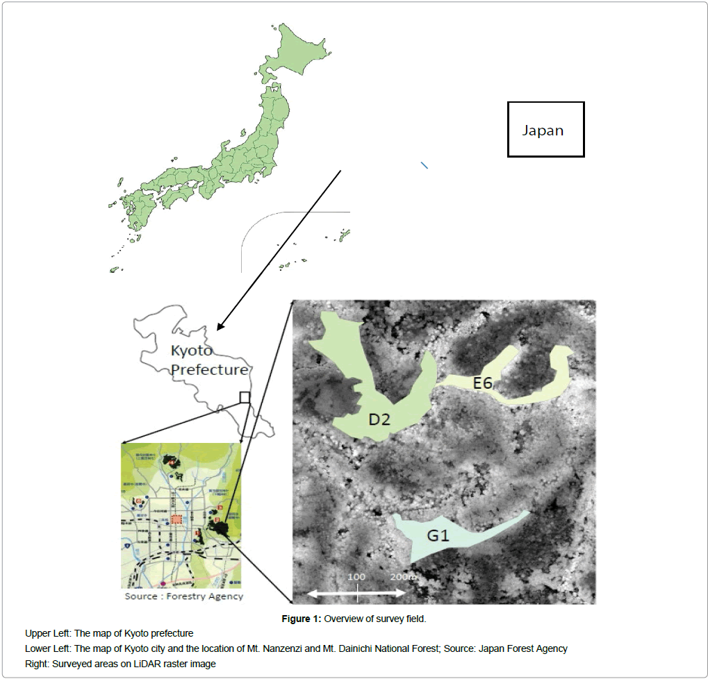
Our study areas include Mt. Nanzenzi and Mt. Dainichi National Forests, which are contiguous to the east urban area of Kyoto City. The compartment numbers we used were 104, 105 and 107 (Figure 1). The area is 46.23 ha and the forests consist of cedar, cypress, red pine, and other deciduous trees. The ages of the trees range from 57 years to 109 years, and the elevation is between 100 and 200 m. We chose three sub-compartments and named them D2, E6, and G1, for convenience (Figure 1). D2 consists of 57-year-old cypress trees that cover 65% of the area (Table 1). These trees are located on gentle slopes near the mountain ridge. E6 is constituted of 103-year-old mixed plantations of cedar and cypress. G1 is a mixed plantation of 109-yearold cypress and red pine trees (Table 1). For E6 and G1, the trees are located along mountain streams or on steep slopes in valleys. The actual stand densities of each survey area were 2,120/ha in D2, 1,100/ha in E6, and 950/ha in G1.
| Sub Compartment | D2 | E6 | G1 |
|---|---|---|---|
| Area (ha) | 3.1 | 1.3 | 1.3 |
| Elevation (m) | 100 | 200 | 100 |
| Slope direction | South | South | West |
| Obliquity | Middle | Middle | Middle |
| Stand Density (/ha) | 2,120 | 1,100 | 950 |
| Dominant | Cypress | Cypress | Cypress |
| Percentage of area | 65% | 90% | 40% |
| Age of tree | 57 | 103 | 109 |
| Sub Dominant | Cedar | Cedar | Red pine |
| Percentage of area | 20% | 10% | 40% |
| Age of tree | 57 | 103 | 109 |
Table 1: The data on Forest register (Kyoto and Osaka Forest management office).
LiDAR (point cloud) data
LiDAR data and aerial photographs were acquired on November 24 and 26, 2013, using a helicopter-borne laser scanner (HARRIER56, Trimble) operated by Asia Air Survey, Japan. LiDAR data were acquired using the following specifications: Average flight speed was 20 m/s at a flight altitude between 550 m and 1360 m above sea level. Pulse frequency was 120 kHz, scan frequency was 44.74 kHz, and scan angle was ±30°. The overlap between courses was over 50%. The LiDAR system registered two echoes of the laser beam – the first and the last pulse. The laser sampling density of the LiDAR data was configured for acquiring >4 points/m2. A Global Navigation Satellite System (GNSS)-based control station was located at Kyoto Sakyo 2, code EL05235466102. The orthophoto created from aerial photographs was used to confirm tree locations on the image of Fusion/LDV display.
Fusion/LDV
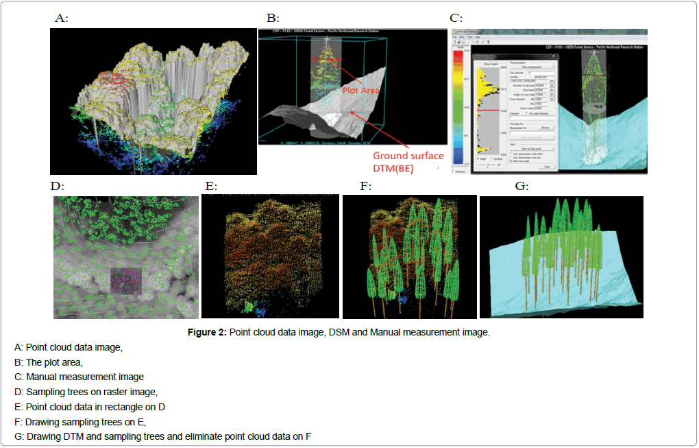
Fusion/LDV is free software that was developed as a forest inventory analysis tool by Robert J. McGaughey at the USDA Forest Service North Pacific Research Station. LiDAR Data Viewer (LDV) can visualize point cloud data in three dimensions are shown in Figure 2A and can measure the tree height, CBH, and CW of every individual tree (Figure 2B and Figure 2C). It can also record this data in the CSV format. Furthermore, LDV can determine the location of trees that are extracted automatically from the raster image by the Local Maxima (LM) technique (Figure 2D, green circles). They can also change colors according to the height by extracting a quadrangle or a circle at any point on the image (Figure 2E), overlay tree images on a point cloud image (Figure 2F), and construct a surface image without point cloud data (Figure 2G). The algorithm of the LM technique is used to find the location of a tree and calculate crown width from the Digital Canopy Height Model (DCHM). The location of a tree is identified at the highest point within a variable window (default window size is 3 × 3) with x and y coordinates. After identifying the tree location, its height and CW were calculated. The CW was calculated by using the LM algorithm developed by Popescu and Wynn [12,13], together with the Tree VAW (Vertex Ant Walk) software [14]. The window size was determined by the height of the DCHM surface at the center of the window by the following equation:
A: Point cloud data image,
B: The plot area,
C: Manual measurement image
D: Sampling trees on raster image,
E: Point cloud data in rectangle on D
F: Drawing sampling trees on E,
G: Drawing DTM and sampling trees and eliminate point cloud data on F
Figure 2: Point cloud data image, DSM and Manual measurement image.
Width = A + B*ht + C*ht² + D*ht³ + E*ht4 + F*ht5 (ht: height) (1)
Default values were applicable for metric units: A = 2.51503, B = 0, C = 0.00901, D = E = F = 0. The maximum crown width was computed from 16 radial profiles extracted from the DCHM. The CBH was assigned a half of tree height automatically (Cited from Fusion/LDV Software Manual) [15]. By using MS-DOS commands, we can partition the LiDAR data and generate data (change parameters according to tree types, ages, or tree height with the /Switches command line). Data processed by Fusion/LDV were compatible with ArcGIS.
Methods
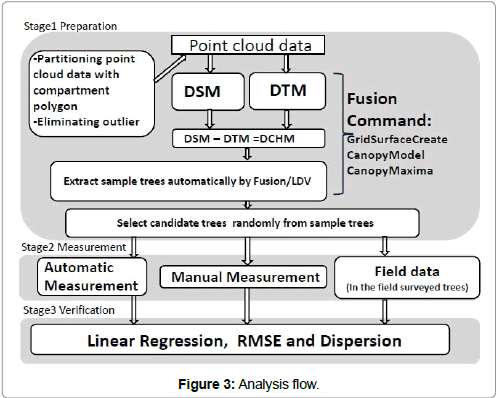
This study involved three major stages. The first stage was the preparation of data for analysis. The second stage was measurement and the third stage was verification of precision (Figure 3). For the preparation of the data, we created a Digital Surface Model (DSM) and a Digital Terrain Model (DTM) from LiDAR point cloud data using Fusion/LDV software. Afterwards, we created a DCHM by subtracting the DTM from the DSM. When the DCHM was created by the (CanopyModel) command of Fusion/LDV, we selected a cell size of 0.5 m because the resolution of pulse density was four points per square meter. That means one pulse was irradiated 0.5 m per square. The filtering range (the range of Local Maxima) was 3 × 3 because it was a default value of the Tree VAW algorithm. The first step was the extraction of sample trees based on the DCHM data using the automatic extraction function (CanopyMaxima) of Fusion/LDV. In addition, the tree height, DBH and CW data of sample trees were measured automatically by (CanopyMaxima). Then we randomly selected candidate trees from the sample. The candidate trees were automatically selected at equal intervals from sample trees table without any other conditions. We used Japanese cypress only for the verification analysis.
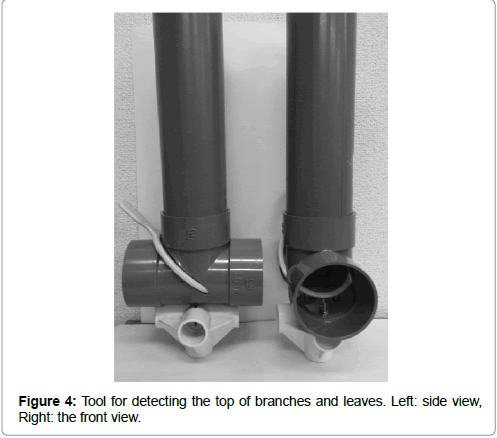
In the second stage, we measured the tree height, CBH (the distance from terrain surface to the lowest branch that had some live leaves), and CW using the following three methods: field survey, automatic measurement, and manual measurement. In the field survey, we registered the position data of the candidate trees on the handy GPS (Garmin-GPSMAP65CSJ) and located them in the field using the GPS. The selected candidate trees were located by stabilizing the GPS at their roots. We identified the trees that can get tree position data as in the field surveyed trees. The tree height and CBH were measured by VERTEX III. The CW was measured by an original tool constructed to detect the tops of branches with leaves (Figure 4). We constructed this tool with a mirror and pipe to find the correspondence point of the tops of branches with leaves, using a perpendicular line created by a string extending from the center of the pipe. CW was defined as a mean of the distance from the trunk to top of branches with leaves in four directions, i.e. north, south, east and west. The accuracy of measurement for this type of tool was verified [16]. Seventy-eight candidate trees were identified in sub-compartment D2, 34 in E6, and 36 in G1 (Table 2). Since we focused on cypress trees among the candidate trees, the number of field surveyed trees was limited to 21 in D2, 16 in E6, and 21 in G1. Surveyed trees were differentiated from the sample trees on the LDV display by manual measurement, and manual measurement plots were set for each surveyed tree. When we manually measured candidate trees, we set a cylindrical area that can change the measurement area of candidate tree. This area was called the measurement plot in Fusin/LDV. After setting the measurement plots, we measured the tree height, CBH, and CW manually by using Fusion/LDV and added the coordinate data for each tree. Then, we recorded these data in CSV format.
| Sub Compartment | D2 | E6 | G1 |
|---|---|---|---|
| Sample trees | 748 | 276 | 233 |
| Candidate trees | 78 | 34 | 36 |
| In the field surveyed trees | 25 | 28 | 28 |
| Cypress trees surveyed | 21 | 16 | 21 |
Table 2: Number of sample, candidate, survey and cypress trees.
In the third stage, we compared the automatic measurements and the manual measurements with the field data by plotting them on a scatter diagram. We also performed statistical tests to calculate the coefficient of determination and the root-mean-square error (RMSE) between the field data and the automatic or manual measurement. Moreover, we drew box plots that indicate the positive or negative differences from the field surveyed data, in order to understand the dispersion of difference. Here, we defined the dispersion as differences between the above mentioned maximum value and minimum value.
Results
Table 2 shows the number of sample, candidate and survey trees. In addition, Table 3 shows the average values of various measurements. For example, the average tree height in D2 was 18.5 m based on field measurement, 18.2 m by automatic measurement, and 19.6 m by manual measurement. Both the manual measurements and the automatic measurements of the crown base height were overestimated compared to the field measurement (Table 3).
| sub compartment |
D2 | E6 | G1 | ||||||
|---|---|---|---|---|---|---|---|---|---|
| (m) | field | automatic | manual | field | automatic | manual | field | automatic | manual |
| height | 18.5 | 18.2 | 19.6 | 26.3 | 27.1 | 26.8 | 25.3 | 24.1 | 25.2 |
| crown base height | 9.0 | 9.1 | 12.3 | 10.9 | 13.5 | 14.9 | 10.4 | 12.0 | 14.2 |
| crown width | 5.7 | 5.1 | 6.9 | 9.2 | 7.5 | 8.4 | 8.8 | 6.2 | 5.9 |
Table 3: Average values by measurement method.
Results of linear regression analysis
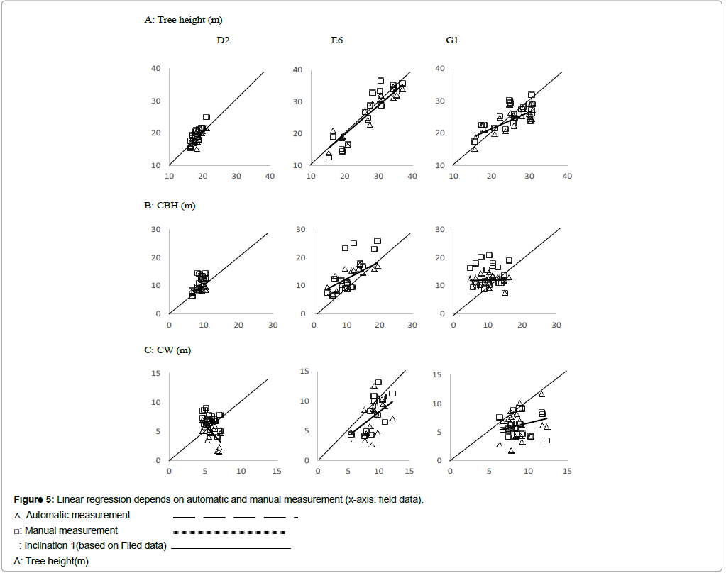
The coefficients determination of the tree heights by both the automatic and manual methods were greater than 0.85 in E6 and between 0.54 and 0.71 in D2 and G1 (Table 4 and Figure 5A). There was significant relation between the reported field measurement and both the automatic and manual measurements in E6, but not for in D2 and G1. The slope of the regression line was slightly under +1 in the case of the automatic measurements (0.99 in D2 and 0.91 in E6). However, the y-intercept of the regression line had a positive value (Table 4). On the other hand, the slope of the regression line was greater than +1 with a negative y-intercept in the case of the manual measurements (1.41 in D2 and 1.15 in E6). The slope of the regression line was greater than 0.5 and the y-intercept was greater than 10 in both the automatic and manual measurements of G1.
|   |  Sub Compartment |
  | D2 | E6 | G1 |
|---|---|---|---|---|---|
| Linear Regression | Height | Automatic | 0.99x + 0.74 | 0.91x + 1.57 | 0.52x + 10.82 |
| Manual | 1.41x – 5.99 | 1.15x - 4.27 | 0.54x + 11.64 | ||
| Crown Base Height | Automatic | 0.41x + 5.55 | 0.60x + 6.48 | 0.02x + 11.84 | |
| Manual | 1.41x – 1.07 | 1.14x + 2.12 | 0.004x + 13.30 | ||
| Crown Width | Automatic | -1.34x + 12.82 | 0.80x + 0.16 | 0.33x + 3.25 | |
| Manual | -0.86x + 11.80 | 1.27x – 3.73 | 0.06x + 5.91 | ||
| Coefficient of Determination |
Height | Automatic | 0.5590 | 0.8699 | 0.5848 |
| Manual | 0.7076 | 0.8752 | 0.5420 | ||
| Crown Base Height | Automatic | 0.3351 | 0.5911 | 0.0013 | |
| Manual | 0.4451 | 0.5498 | 0.0008 | ||
| Crown Width | Automatic | 0.3782 | 0.1988 | 0.0483 | |
| Manual | 0.7153 | 0.4625 | 0.0030 |
Table 4: Linear Regression and Coefficient of Determination.
With regard to the CBH, the coefficient of determination was less than 0.6 both in the automatic and manual measurements of D2 and E6, and nearly zero in G1 (Table 4). The slope of the regression line was less than 0.6 and the y-intercept was greater than 5 in the automatic measurements of D2 and E6. For the manual measurements, the slopes of the regression line were 1.41 in D2 and 1.14 in E6. In G1, for both the automatic and manual measurements, the slope of regression line was nearly zero and the y-intercept was greater than 10.
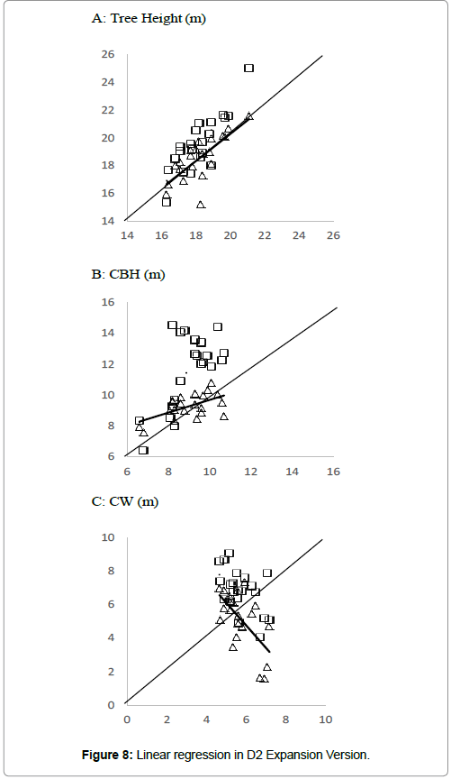
While regarding the CW, the coefficient of determination was also less than 0.72 for both the automatic and manual measurements at each field. The coefficient of determination was as small as the crown base height and there was no significant relation between the results in G1. Linear regression analysis exhibited a negative relation, with a slope of −1.34 for the automatic measurements and −0.86 for the manual measurements in D2. In E6, the slope was 0.8 for the automatic measurements and 1.27 for the manual measurements, and in G1, the slope was less than 0.33 for both the automatic and manual measurements.
Dispersion of differences
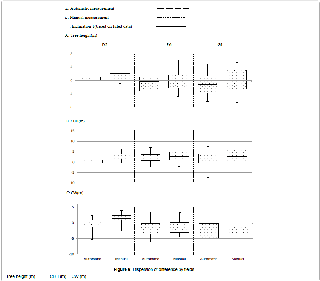
According to the box plot, the dispersion of difference of the tree heights was less than 5 m in D2, but it was greater than 8 m in E6 and G1 in both the automatic and manual measurement cases. In the case of CBH, the dispersion of differences was considerable in E6 (<15 m) and in G1 (<20 m), but relatively small in D2 (<6 m) for the manual measurement. The CBH had a tendency to overestimate in all stands (D2, E6 and G1). In terms of CW, the dispersion of difference was about 10 m in E6 for the automatic measurement and in G1 for the manual measurement. The others are mostly 7 m, which exhibited small differences. However, the dispersion of difference tended to overestimate the CW in D2 whereas underestimated it in E6 and G1 (Figure 6).
RMSE
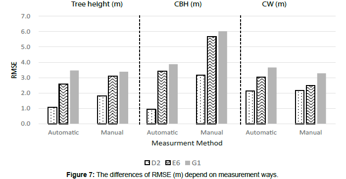
The RMSE of the differences in tree heights was less than 2 m in D2 and around 3 m in E6 and G1. The RMSE of the differences in the CBH was less than 1 m in D2, but approximately from 3 m to 6 m in the other cases. The RMSE of the CW was between 2.1 m and 3.7 m. RMSE of D2 was smaller than the others in all cases (Figure 7).
Discussion
In order to examine the efficiency of Fusion/LDV, the values of automatic and manual measurements on tree height, CBH and CW were compared with the surveyed value in the field by using linear regression, dispersion, and RMSE.
Tree height
The results of the automatic and manual measurements were relatively significant with average differences of ±1.2 m, and with slopes of the regression line of nearly equal to one. However, the dispersion difference (Figure 6) was larger in E6 and G1 (approximately 8 m) than in D2 (approximately 5 m). The result of the RMSE analysis confirmed the same tendency. The larger differences in E6 and G1 might be because the age of both forest stands was more than 100 years. In older stands, younger or suppressed trees, which show large size variation compared to the average tree height of a 100-year-old tree, could be of mixed species because of the passage of time allowing opportunity for new plants to invade than in younger stands. When measuring a different tree by the precision of the GPS as one of possibilities, it is considered that an error occurred. It can think the difference is small even if the tree height of the different tree is measured, because the tree height difference between the individuals is small at D2. Another factor to be considered might be the difference in the locations of surveyed trees. In D2, the surveyed trees are located on or near the ridge, while in E6 and G1, they are located near a mountain stream, valley, or at a hillside, which may result in some topographical error [17].
CBH
on the results of the average difference (Table 3), scatter diagrams, linear regression (Figure 5), and box plots (Figure 6), the CBH tended to be overestimated for both the manual and automatic measurements in all fields. The average ratio of CBH to tree height of all trees was 0.49 in D2, 0.42 in E6, and 0.42 in G1. In automatic measurement, CBH is computed the half of tree height. The reason for this overestimation might be measurement error. The automatic measurement of Fusion/LDV for the CBH is set at just half of the tree height, which is considered to be based on the North America scenario. However, the CBH of the Japanese plantation has changed greatly by pruning. In most cases, the CBH is longer than the half of the height. But according to the field survey results, CBH was shorter than the half of the height in every survey site. In this national forest, there were no records of pruning or other maintenances. Accordingly, it is possible that the length of branches with leaves remained under the half of tree height. In the case of manual measurements, it was difficult to find the lowest crown height by decreasing the number of passes or return pulse by branches and leaves. The correct shape cannot be plotted on the personal computer screen. The results indicate that the operator tended to choose the lower point, which did not really indicate the lowest point of the crown.
CW
Based on the results of the average difference (Table 3), scatter diagrams, linear regression (Figure 5), and the box plots (Figure 6), for E6 and G1, the result of the CW was underestimated for both the automatic and manual measurements. However, the D2, manual measurements were overestimated, and its median value was near zero for the automatic measurements.
The tree VAW algorithm calculates the CW as the distance from the top of the tree to the lowest height of the crown between adjacent trees. This method was applied because the extraction of the top of the branches with leaves is very difficult where the crowns overlap [13]. The accuracy of CW calculation depends on the variable-size of evaluation window [15]. It is recommended to use setting of the crown width added to local tree crown circumferences. In the case of manual measurements, it was difficult to detect the heap of branch by determining the radius of the measurement area using visual observation on computer screen. Thus, it could be said that the under- and overestimated CW results achieved when using both the manual and automatic measurements were due to the difficulties experienced in detecting the correct branch heap when the tree crowns overlapped.
The differences by fields
Comparing all the results parameters among the study fields, the differences in D2 results tended to be smaller compared to E6 and G1 results (Figure 6-8) (Tables 3 and 4). This might be due to the age of the stands. The age of the trees in E6 and G1 were > 100 years. On the other side, the trees in D2 were 57 years old. The age difference led to the crown size difference; the crown size of D2 might be smaller than those of E6 and G1. Thus, it is better to change the cell size and filtering size according to the crown size when creating the DCHM [13]. However, when the DCHM was created, we selected a cell size of 0.5 m and the filtering range was 3 × 3 by the (CanopyModel) of Fusion/LDV with 4 points/m2 of laser sampling density. There is a possibility that the cell size and the filtering size did not match the size of the crown of E6 or G1. Further investigation is required to understand the effect of the cell size and filtering size on the analysis of individual trees in different aged stands using LiDAR data. In terms of the stand density, this study results indicate that there were not significant differences in the stand density with average tree height. However, we need more research with diverse forest conditions.
Conclusion
In this study, we applied the measurement functions of Fusion/LDV to Japanese forest stands using point cloud data from LiDAR, and compared the results of the software’s automatic and manual measurements to field measurement results. The following parameters were verified: tree height, CBH, and CW. The results of the verification showed that the estimations of tree heights by both automatic and manual measurements of Fusion/LDV had relatively high precision in average tree heights. However, the results of both the automatic and manual measurements were not significant for individual tree height, CBH and CW in diverse forest conditions. For the ITD, CBH, and CW, further research focusing on the methods of analysis is required. We consider Fusion/LDV as a partially efficient tool that can only be used for detecting the average tree height in the overcrowded Japanese forest stands. We need further research not only to analyze the characteristics of the LiDAR data such as cell size and window size but also to examine the LiDAR analysis method.
Acknowledgment
The LiDAR data and study area were made available by the Kyoto-Osaka District Forest Office, Kinki Chugoku Regional Forest Office, and Forestry Agency. We greatly appreciate their contributions. This work was supported by JSPS KAKENHI (grant number 24580225).
References
- Akiyama Y (1999) Activation Method of High-density topography measurement with Airborne RASER for afforestation projects. Afforestation Research Reports 37: 343-350.
- Næsset E (1997a) Determination of mean tree height of forest stands using airborne laser scanner data. J Photogramm Remote Sens 52: 49 -56.
- Næsset E (1997) Estimating timber volume of forest stands using airborne laser scanner data. Remote Sens Environ 61: 246-253.
- Maganussen , Boudewyn (1998) Derivations of stand heights from airborne laser scanner data with canopy-based quantile. Can J For Res 28: 1016-1031
- Lefsky MA, Cohen WB, Acker SA, Parker GG, Spies TT, et al. (1999) Lidar remote sensing of canopy structure and biophysical properties of Douglas-fir western hemlock forests. Remote Sens Environ 70: 339-361.
- White JC, Wulder MA, Varhola A, Vastranta M, Coops NC, et al. (2013) A Best Practice Guide for Generating Forest Inventory Attributes from Airborne Laser Scanning Data Using an Area-Based Approach. For Chron 89: 722-723.
- Næsset E (2002) Predicting forest stand characteristics with airborne scanning laser using a practical two-stage procedure and field data. Remote Sens Environ 80: 88-99.
- Breidenback J, Næsset E, Lien V, Gobakken T, Solberg S (2010) Prediction of species specific forest inventory attributes using a nonparametric semi-individual tree crown approach based on fused airborne laser scanning and multispectral data. Remote Sens Environ 114: 911-924.
- Vauhkonen J, Ene LG, Heinzel J, Holmgren J, Piktänen J, et al. (2012) Comparative testing of single-tree detection algorithms under different types of forest. Forestry 85: 27-40.
- Kaartinen H, Hyyppa J, Yu XW, Vastaranta M, Hyyppa H, et al.(2012) An International Comparison of Individual Tree Detection and Extraction Using Airborne Laser Scanning. Remote Sens 4: 50-974.
- Mitchell B, Walterman M, Mellin T, Wilcox C, Lynch AM (2012) Mapping vegetation structure in the Pinaleño Mountains using lidar – Phase 3: forest inventory modeling. RASC-10007-RPT1.
- Popescu SC, Wynne RH, Nelson RF (2002) Estimating Plot-level tree heights with lidar: local filtering with a canopy-height based variable window size. Computers and Electronics in Agriculture 37: 71-95.
- Popescu SC, Wynne RH (2004) Seeing the trees in the Forest: Using Lidar and Multispectral Data Fusion with Local Filtering and Variable Window Size for Estimating Tree Height. Photogramm Eng Rem S70: 589-604.
- Kini AU, Popescu SC (2004) Tree VAW: A versatile tool for analyzing forest canopy Lidar data – a preview an eye towards future. ASPRS 2004 Fall Conference,12–16 September 2004, USA.
- McGaughey RJ (2014) Fusion/LDV: Software for LiDAR Data Analysis and Visualization, March 2104 – Fusion Version 3.42
- Takahashi E, Takahashi S, Takeuchi M (2015) Development of a new tree crown measurement tool, the Ten-bou-kyou, and a case study of its accuracy and prediction. Applied Forest Science 24: 29 -33.
- Hirtata Y (2005a) Influence of transmittance and sampling density of laser beams in forest measurement of a Cryptomeria japonica stand with an airborne laser scanner. JPN J For Plann 39: 81-95.
 Spanish
  Chinese
  Russian
  German
  French
  Japanese
  Portuguese
  Hindi
Hindi 