Spanish
  Chinese
  Russian
  German
  French
  Japanese
  Portuguese
  Hindi
Hindi Research Article, Res J Econ Vol: 1 Issue: 1
Long-Run Relation and Short-Run Dynamics in U.S. Energy Demand: Evidence from Panel Data across Energy Sources and User Ends
Hassan Mohammadi* and Monalisa Kulkarni
Department of Economics, Illinois State University, USA
*Corresponding Author : Hassan Mohammadi
Department of Economics, Illinois State University, Normal, IL 61790-4200, USA
Tel: 309(438)7777
E-mail: hmohamma@ilstu.edu
Received: October 13, 2017 Accepted: October 25, 2017 Published: November 01, 2017
Citation: Mohammadi H, Kulkarni M (2017) Long-Run Relation and Short-Run Dynamics in U.S. Energy Demand: Evidence from Panel Data across Energy Sources and User Ends. Res J Econ 1:1.
Abstract
Long-run relations and short-run dynamics of demand for energy, electricity and natural gas are examined using panel data for 48 U.S. states over 1970-2013 periods across the residential, commercial and industrial sectors. Five noteworthy points are evident: (1) Tests of cointegration, which account for cross-sectional dependency, suggest the existence of stable demand functions across the three sectors. (2) Estimates of price and income elasticities have the correct signs and are significant across most sectors. (3) Energy demand is both price and income inelastic in the long-run across different types of energy and end-use sectors. (4) There is no evidence of substitutability or complementarity between electricity and natural gas. (5) There is no evidence that the magnitude of price elasticity varies by extend of the market. And, (6) the estimated error-correction model suggests long-run causality from explanatory variables to energy. This finding is robust across energy types and end-use sectors.
Keywords: Energy demand; Price elasticity; Income elasticity; Panel cointegration; Common-correlated effect mean-group estimators
Introduction
Price and income elasticities of demand for energy and its byproducts are crucial in empirical analysis of energy markets as well as in developing effective energy-related price and income policies. More specifically, price and income elasticities are important for at least three reasons: First, they are the necessary ingredient for effective forecasts of future energy demand. These forecasts are in turn, necessary for investment and development of future energy infrastructure and transmission systems. Second, price elasticities capture the responsiveness of energy demand to changes in price. As such, they are necessary for the development of demand management policies and appropriate tax and subsidy programs. Third, income elasticities capture the responsiveness of energy demand to changes in income. As such, they are useful in forecasting energy demand at different levels of income, and in devising appropriate energy income policies. Thus, it is no surprise that a growing body of literature has been devoted to estimate price and income elasticities of demand for various types of energy. The primary purpose of this study is to estimate price and income elasticities of demand for three types of energy – total energy, electricity, and natural gas - in aggregate as well as across three user-ends in the U.S., namely the residential, commercial and industrial sectors. We carry out the empirical analysis with panel data covering the 48 contagious states over 1970-2013. The study attempts to answer four research questions: First, what are the magnitudes of price and income elasticities for different types of energy and across different user-ends? In particular, how sensitive is energy demand to changes in price and income? Second, does the size of price elasticity vary by the extend of the market? More specifically, does the magnitude of the price elasticity increase for more specific energy types and for specific user-ends? See for example, Mankiw’s [1] Principles of Economics. According to Mankiw, the price elasticity of demand depends on the extend of the market. Narrowly defined markets tend to have more elastic demand than broadly defined markets. Third, how do our empirical results compare with those of previous studies? And fourth, what are policy implications of our findings? In particular, how do these findings help develop policies regarding energy markets?
The remainder of the paper is organized as follows. Section 2 provides a brief overview of relevant empirical literature. Section 3 describes our empirical model as well as the estimation method. Section 4 provides a brief description of the variables, data sources, as well as a highlight of their simple statistics. Section 5 reports the estimation results and tests of causality. Section 6 provides a summary of the main findings and major conclusions.
Previous literature
A conventional energy demand model depicts the relationship between the quantity of energy demanded and its determinants such as income, own price, price of substitutes and complements as well as other explanatory variables. There have been three motivations for undertaking energy demand analysis: First, to convey information about the behavior of demand, its functional form, its determinants, and the degree of responsiveness to each determinant. Second, to develop forecasts of future energy demand, which is necessary for future capacity building and infrastructure development. Third, to help devise effective price and income policies related to energy markets. Given its vast literature, this section reviews a representative sample of relevant studies.
Taylor [2] provides an early survey of electricity demand in residential, commercial, and industrial sectors. His reported price elasticities vary between short- and long-run as well as across enduse sectors. For residential sector, short-run price elasticity ranges between –0.13 and –0.90 while long-run price elasticity varies from zero to –2.00. For commercial sector, a point estimate of price elasticity is –0.17 in the short-run, and reaches -1.36 in the long run. Bohi and Zimmerman [3] provide a detailed review of demand for electricity, natural gas, and fuel oil across residential, commercial, and industrial sectors. They report a consensus estimate for the price elasticity of residential electricity demand of –0.2 in the short run and –0.7 in the long run. For electricity demand in the commercial sector, however, price elasticities are highly variable and thus unreliable. For natural gas demand in the residential sector, they report consensus values of –0.2 in the short run and –0.3 in the long run.
A substantial amount of effort in the literature has been directed to sort out econometric modeling techniques that better identify the relationship between energy demand and its determinants. The importance of these studies hinges on extrapolating precise economic information such as price and income elasticities. These studies differ significantly as they improvise in terms of model specification, choice of variables as determinants of demand, estimation techniques and sample period. Using data as the criteria, previous literature can be classified into two broad categories -- those using aggregate (nationwide, state or regional level) data, and those using household level data. Espey and Espey [4] provide a meta-analysis of over 100 studies. Alberini et al. [5] contains a good comparison of 17 more recent studies.
The first set of studies uses macro level U.S. data to fit energy demand functions and estimate the corresponding price and income elasticities. These studies have the advantage of providing price and income elasticities for both the long- and short-run. The estimated elasticities vary widely due to the diverse nature of data (mostly panel and time-series), the extend of the variability in price and income, and the sample period. Halvorsen [6], Houthakker [7], Maddala et al. [8], Bernstein and Graffin [9], Paul et al. [10], Alberini and Filippini [11] use state level panel data along with alternative dynamic adjustment models to estimate energy demand functions. The findings from these studies suggest that demand is relatively price insensitive in the short-run. However, the estimates of the long-run price elasticity are sensitive to the specific estimation procedure.
Time-series analyses of electricity demand at the macro level include, Beenstock et al. [12], Kamerschen and Porter [13] and Hotledahl and Joutz [14]. These studies relate electricity demand to a variety of economic, demographic and meteorological variables. Dergiades and Tsoulfidis [15] report electricity price elasticity of -0.386 in the short-run and -1.06 in the long-run using U.S. aggregate data. Kamerschen and Porter [13] report price elasticities in the range of -0.85 to -0.94. Liu [16] examines the own- and cross-price elasticities of demand for natural gas in residential, commercial and industrial sectors for Department of Energy (DOE) regions in the U.S. using a simultaneous equation model with data from 1967 to 1987. The findings suggest that natural gas is much more priced elastic in the long-run than the short-run; the industrial sector is the least price responsive; and there are significant variations in the estimated elasticities across regions and sectors.
The second category of studies employs micro-level (household) data that are limited in either time coverage or geographic scale and have imputed price and quantity data. Hirst et al. [17] estimate priceand income-elasticities of electricity demand using a cross-section of U.S. households from the National Interim Energy Consumption Survey (NIECS). Their findings are consistent with the view that demand is less price- and income-elastic in the short-run than the long-run. Quigley and Rubinfeld [18] find similar results using a crosssectional data from the 1980 American Housing Survey. Metcalf and Hassett [19] use the 1984, 1987 and 1990 waves of the Department of Energy’s Residential Energy Consumption Survey (RECS) to examine homeowner’s insulation investments. Their findings suggest the price elasticity of electricity ranges from -0.73 to -1.16. Finally, a recent study by Alberini and Filippini [11] uses data from the American Housing Survey on household electricity expenditure. The study accounts for potential measurement errors and simultaneity bias in the model. Broadly speaking, studies with household data generally produce smaller price- and income-elasticities, with long-run price elasticities in the range of 0 to −0.6 and the long-run income elasticity in the range of 1.0 to 2.0 respectively. A number of studies (Bernard et al., Garcia-Cerrutti, Reiss and White) [20-22] have examined household demand for energy. However, these studies are restricted to limited geographical areas rendering them inapplicable to broader areas.
Apart from the U.S., several studies have examined energy demand in other countries. Narayan et al. [23] examine the income and price elasticities of residential demand for electricity in G-7 countries using panel cointegration tests with data over 1980-2008. Their findings suggest that long-run residential electricity is price elastic but income inelastic. Lee and Lee [24] investigate the demand for electricity and total energy in OECD countries using panel cointegration tests with data over 1978-2004. Their findings suggest that total energy demand is price and income inelastic. However, electricity demand is income elastic but price inelastic. Blazquez et al. [25] examine the residential demand for electricity for 47 Spanish provinces using a dynamic partial adjustment approach over 2000-2008. Their findings suggest price-inelastic demand in both short- and long-run. Their findings also suggest significant impact of weather on the electricity demand.
A large number of studies have focused on electricity demand in the residential sector, which comprises a large component of electricity market. Silk and Joutz [26], Beenstock et al. [27], Fatai et al. [28], Hotledahl and Joutz [14], Hondroyiannis [29], Halicioglu [30] and Zachariadis and Pashourtidou [31] are examples of this line of research.
In summary, there is no consensus on point estimates of price and income elasticities for energy demand and its components. The estimated elasticities vary by the choice of the model, the data, sample period, and the empirical method. Thus, we contribute to the literature by reexamining the sensitivity of energy (total energy, electricity, and natural gas) demand to changes in price and income across the three user-ends, namely residential, commercial and industrial sectors.
Theoretical Model and Empirical Method
general state-level energy demand function can be characterized as,
![]() (1)
(1)
where, Qit is per capita energy demand in state i at time t; Yit is its real per capita income; PAit is its own real price; PBit is the real price of an alternative (substitute or complement) energy; HDDit and CDDit denote the heating-degree- and cooling-degree-days. Four points regarding our empirical work is noteworthy: (1) We consider three alternative measures of Qit: total energy (EN), electricity (EL), and natural gas (NG). (2) For each of the three measures, we estimate demand functions for aggregate as well as in three enduse residential, commercial, and industrial sectors. (3) In modeling electricity demand, we use real natural gas prices as the PBit variable; in modeling natural gas demand, we use real electricity prices as the PBit variable; and in modeling total energy demand, we assume there is no price substitute. (4) For analyses at the sect oral level, PAit and PBit would refer to sector-specific real prices.
Assuming a log-linear relation between Qit and the right-handside variables, the demand function can be written as,
![]() (2)
(2)
where, lower case letters are the natural logs of the variables in (1), εit is the idiosyncratic error term for the ith state at time t, αi (i =1,…,N), are state-specific intercepts, dt are dummy variables, which take the value of one for time (t =1, …, T), and zero otherwise; and βi, γi, δi, θi, ωi are the corresponding elasticities. Economic theory suggests , βi > 0, γi < 0, θi > 0, ωi > 0, but δi may be of either signs as it depends on the substitutability or complementarity nature of the two energy sources.
As Pesaran [32], Mohammadi and Amin [33] and Chintrakarn et al. [34] point out, estimation of parameters in equation (2) requires careful attention to three important issues: First, tests of cointegration require income, price and energy demand variables to be non-stationary in level, stationary in first-difference, and have a stationary linear combination (i.e., the error term must be stationary). Stationarity of the error term implies that no relevant non-stationary variable is omitted from the model. If the true cointegrating model includes other non-stationary variables, then their omission would produce a non-stationary error-term and makes detection of cointegration difficult. Second, states vary in size, income level, geographical location, resources, etc. Thus price and income elasticities may vary significantly across states and treating them equal might produce inconsistent and potentially misleading estimates (Pesaran et al.,) [35]. Thus, estimation of equation (2) requires proper account of cross-state parameter heterogeneity. Third, variables in the energy demand model may be subject to common shocks, and subject to cross-sectional dependency. Thus, estimation of equation (2) requires proper account of cross-sectional dependency in the variables.
In order to estimate the long-run price and income elasticities of energy demand we utilize the common-correlated-effect meangroup estimator (CCEMG) proposed by Pesaran [32]. This procedure accounts for the existence of unobserved common factors across states by augmenting equation (2) with cross-sectional averages of all variables as additional regressors. Kapetanios et al., [36]
![]() (3)
(3)
Where, ![]()
The common correlated effect (CCE) estimator for the ith state’s slope coefficients proposed by Pesaran [32] is,
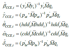
Where, ![]() is a T × 6 matrix of observations on
is a T × 6 matrix of observations on ![]() . The CCE estimators are consistent irrespective of common factor stationarity.
. The CCE estimators are consistent irrespective of common factor stationarity.
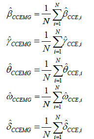
The CCEMG estimators, which account for cross-sectional heterogeneity and dependency, are obtained as simple average of the estimated coefficients across states,
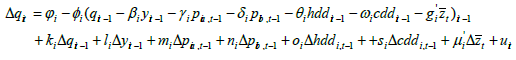
Next, to examine the dynamics of energy demand and to test for long- and short-run causalities, we estimate the corresponding panel vector-error-correction model (which also accounts for common factors) following Moscone and Tosetti [37],
 (4)
(4)
Where, the term in parentheses is lagged adjusted equilibrium error, and
![]()
Equation (4) reflects the dynamics of energy demand to changes in income, own- and cross-prices, as well as the heating- and coolingdegree- days. We estimate equations (3) and (4) for three types of energy (total energy, electricity, and natural gas) as well as across the three residential, commercial and industrial sectors.
Data
The study uses annual data for 48 U.S. states over 43 years (1970- 2013). We use data on per capita consumption of total energy, electricity and natural gas as well as their respective measures in residential, commercial and industrial sectors (in million BTU). The state data for real income is obtained by dividing state nominal income with the consumer price index. To make the analysis comparable across states, all variables are transformed into per capita using state population, and are in logarithmic form.
Data for per capita state nominal income (in $) and state population are obtained from the Bureau of Economic Analysis (BEA). Data for consumption of total energy, electricity, and natural gas, their respective user-end consumption in residential, commercial and industrial sectors, prices of energy, electricity and natural gas and data for heating- and cooling-degree-days are obtained from the Energy Information Administration (EIA) State Energy Data System (SEDS).
Table 1 presents simple statistics for per capita consumptions of energy, electricity, and natural-gas ![]() , their respective average real prices
, their respective average real prices ![]() , average real per capita income
, average real per capita income ![]() , and average heatingand cooling-degree-days across the 48 states over 1970-2013 sample period, A review of summary statistics reveals six points. First, energy consumption is close to ten times higher than electricity consumption and more than four times higher than natural gas consumption. Second, energy consumption has the highest variability followed by natural gas and electricity consumption. Third, all three measures of energy consumption are skewed to the right, and have peaks higher than a normal distribution. Fourth, natural gas is 50% cheaper than total energy and 75% cheaper than electricity. Fifth, all three energy prices are skewed to the right. However, there is no evidence of kurtosis as the three values are close to 3.00 which are for a normal distribution. Sixth, average per capita real income is $14,542 with standard deviation of $3,415, which is positively skewed and has a peak higher than a normal distribution. Seventh, average heatingdegree- days (HDD) are about five times higher than the average cooling-degree-days (CDD). HDD is negatively skewed with a peak below a normal distribution while HDD is positively skewed and has a peak higher than a normal distribution.
, and average heatingand cooling-degree-days across the 48 states over 1970-2013 sample period, A review of summary statistics reveals six points. First, energy consumption is close to ten times higher than electricity consumption and more than four times higher than natural gas consumption. Second, energy consumption has the highest variability followed by natural gas and electricity consumption. Third, all three measures of energy consumption are skewed to the right, and have peaks higher than a normal distribution. Fourth, natural gas is 50% cheaper than total energy and 75% cheaper than electricity. Fifth, all three energy prices are skewed to the right. However, there is no evidence of kurtosis as the three values are close to 3.00 which are for a normal distribution. Sixth, average per capita real income is $14,542 with standard deviation of $3,415, which is positively skewed and has a peak higher than a normal distribution. Seventh, average heatingdegree- days (HDD) are about five times higher than the average cooling-degree-days (CDD). HDD is negatively skewed with a peak below a normal distribution while HDD is positively skewed and has a peak higher than a normal distribution.
| Mean | S.D. | Skewness | Kurtosis | |
|---|---|---|---|---|
| Total Energy | ||||
| 370.66 | 158.67 | 2.54 | 10.34 | |
| 6.89 | 1.86 | 0.53 | 2.94 | |
| Electricity | ||||
| 38.48 | 13.35 | 0.92 | 4.75 | |
| 14.16 | 4.32 | 0.55 | 2.84 | |
| Natural Gas | ||||
| 91.41 | 93.55 | 3.46 | 17.61 | |
| 3.46 | 1.24 | 0.35 | 2.93 | |
| Common for all | ||||
| 14542.50 | 3415.08 | 0.61 | 3.13 | |
| 5236.93 | 2046.84 | -0.13 | 2.34 | |
| 1093.72 | 784.59 | 1.18 | 3.89 | |
Table 1: Summary Statistics- Average per capita consumption of energy, electricity and natural gas and their respective prices and income per state.
Empirical Results
Test of cross-sectional dependency
Table 2 reports the results of test of cross-sectional dependency along with estimates of the cross-sectional parameters for energy, electricity and natural-gas consumption across the residential, commercial and industrial user-ends. Evidence overwhelming rejects the null hypothesis of cross-sectional independence for each variable for the whole sample as well as across the three user-ends. For per capita energy, commercial sector has the highest cross-state correlation relative to the other two sectors. For per capita electricity and natural-gas, residential sector has the highest correlation compared to commercial and industrial sectors.
| (A) | Total Energy | Residential | Commercial | Industrial | ||||
|---|---|---|---|---|---|---|---|---|
| CDP | CDP | CDP | CDP | |||||
| Δqit | 0.17 | 37.43*** | 0.36 | 78.43*** | 0.41 | 91.12*** | 0.27 | 59.68*** |
| Δpa,it | 0.42 | 92.55*** | 0.51 | 111.33*** | 0.89 | 195.03*** | 0.66 | 144.34*** |
| ΔYit | 0.64 | 141.18*** | 0.64 | 141.18*** | 0.64 | 141.18*** | 0.64 | 141.18*** |
| Δhddit | 0.46 | 101.15*** | 0.46 | 101.15*** | 0.46 | 101.15*** | 0.46 | 101.15*** |
| Δcddit | 0.35 | 76.66*** | 0.35 | 76.66*** | 0.35 | 76.66*** | 0.35 | 76.66*** |
| (B) | Electricity | Residential | Commercial | Industrial | ||||
| Δqit | 0.39 | 86.36*** | 0.32 | 70.37*** | 0.23 | 49.69*** | 0.24 | 53.69*** |
| Δpa,it | 0.34 | 73.72*** | 0.27 | 59.00*** | 0.26 | 57.34*** | 0.35 | 76.56*** |
| Δpb,it | 0.69 | 151.31*** | 0.59 | 130.55*** | 0.60 | 131.76*** | 0.59 | 129.97*** |
| (C) | Natural Gas | Residential | Commercial | Industrial | ||||
| Δqit | 0.22 | 48.56*** | 0.39 | 86.69*** | 0.19 | 40.79*** | 0.21 | 45.81*** |
| Δpa,it | 0.69 | 151.31*** | 0.59 | 130.55*** | 0.60 | 131.76*** | 0.59 | 129.97*** |
| Δpb,it | 0.34 | 73.72*** | 0.27 | 59.00*** | 0.26 | 57.34*** | 0.35 | 76.56*** |
Table 2: Tests of cross-sectional dependency in growth rates of per capita consumption of total energy, electricity, natural gas, their respective real prices, real income, and heating- and cooling-degree-days.
Test of unit roots
Table 3 reports the Maddala and Wu (MW) and Pesaran (CIPS) tests of panel unit roots with zero and one auxiliary regressors (see, Maddala and Wu; Pesaran) [38,39]. The MW test does not account for cross-sectional dependency, while the CIPS does. Thus, given the earlier evidence in favor of cross-sectional dependency reported in Table 2, the CIPS test is more appropriate. Nevertheless, both tests reach similar conclusions: all variables are non-stationary at conventional 5 percent significance level for aggregate measures of energy, electricity and natural-gas as well as across the residential, commercial and industrial sectors. Thus, for the remainder of the analysis, we assume that variables are non-stationary in level and stationary in first-difference form, and proceed to tests of cointegration.
| Residential | Commercial | Industrial | ||||||
|---|---|---|---|---|---|---|---|---|
| CADF(0) | CADF (1) | CADF(0) | CADF (1) | CADF(0) | CADF (1) | CADF(0) | CADF (1) | |
| A. Total Energy | ||||||||
| Maddala and Wu (MW) | ||||||||
| q | 119.66* | 111.07 | 379.83*** | 220.17*** | 91.05 | 106.24 | 110.96 | 103.28 |
| pa | 66.36 | 99.21 | 63.71 | 95.9 | 23.68 | 40.3 | 61.4 | 80.62 |
| y | 74.2 | 179.18*** | 74.2 | 179.18*** | 74.2 | 179.18*** | 74.2 | 179.18*** |
| hdd | 1050.14*** | 725.46*** | 1050.14*** | 725.46*** | 1050.14*** | 725.46*** | 1050.14*** | 725.46*** |
| cdd | 1708.53*** | 1090.15*** | 1708.53*** | 1090.15*** | 1708.53*** | 1090.15*** | 1708.53*** | 1090.15*** |
| Pesaran (CIPS) | ||||||||
| q | -3.53*** | -1.75** | -8.13*** | -3.19*** | -0.64 | 2.41 | 0.14 | 2.41 |
| pa | -6.74*** | -6.01*** | -6.76*** | -4.60*** | -4.99*** | -3.23*** | -6.19*** | -4.12*** |
| y | 6.93 | 5.48 | 6.93 | 5.48 | 6.93 | 5.48 | 6.93 | 5.48 |
| hdd | -25.05*** | -15.29*** | -25.05*** | -15.29*** | -25.05*** | -15.29*** | -25.05*** | -15.29*** |
| cdd | -28.06*** | -15.82*** | -28.06*** | -15.82*** | -28.06*** | -15.82*** | -28.06*** | -15.82*** |
| B. Electricity | ||||||||
| Maddala and Wu (MW) | ||||||||
| q | 82.74 | 82.35 | 233.99*** | 167.18*** | 62.14 | 71.94 | 127.50** | 151.25*** |
| pa | 66.12 | 98.99 | 58.23 | 89.84 | 62.45 | 83.36 | 75.37 | 112.31 |
| pb | 33.82 | 45.1 | 30.06 | 39 | 30.88 | 44.52 | 42.06 | 53.39 |
| Pesaran (CIPS) | ||||||||
| q | -3.17*** | -1.14 | -8.48*** | -5.44*** | -3.72*** | -4.68*** | -2.17** | -2.32*** |
| pa | -2.29** | -0.74 | -2.30*** | -0.73 | -3.08*** | -0.5 | -1.81** | 0.6 |
| Pb | -7.26*** | -0.71 | -10.12*** | -4.32*** | -9.24*** | -4.58*** | -8.24*** | -1.07 |
| C. Natural Gas | ||||||||
| Maddala and Wu (MW) | ||||||||
| q | 84.93 | 70.4 | 481.37*** | 293.67*** | 259.68*** | 184.66*** | 91.33 | 87.04 |
| pa | 33.82 | 45.1 | 30.06 | 39 | 30.88 | 44.52 | 42.06 | 53.39 |
| pb | 66.12 | 98.99 | 58.23 | 89.84 | 62.45 | 83.36 | 75.37 | 112.31 |
| Pesaran (CIPS) | ||||||||
| q | -5.30*** | -1.81** | -12.06*** | -7.48*** | -6.82*** | -3.14*** | -3.00*** | -1.76** |
| pa | -7.26*** | -0.71 | -10.12*** | -4.32*** | -9.24*** | -4.58*** | -8.24*** | -1.07 |
| pb | -2.29** | -0.74 | -2.30** | -0.73 | -3.08*** | -0.5 | -1.81** | 0.6 |
Table 3: Tests of panel unit roots.
Tests of cointegration and estimates of the long-run price and income elasticities
Table 4 report the results of CIPS panel cointegration tests, the estimates of price and income elasticities for energy, electricity and natural gas in total as well as in the three sectors (residential, commercial and industrial). As reflected in panel A of the Table, there is overwhelming support for the existence of cointegration in demand equations for total energy as well as in their three end-use sectors. The null hypothesis of panel unit roots in residuals of the demand equations is rejected for total energy and its end-use sectors. Estimates of own price elasticity ![]() are negative and significant for total energy and its end-use sectors. Energy demand is price inelastic. However, the values of the elasticity vary from -0.208 in residential sector to -0.520 in the commercial sector. Estimates of income elasticity
are negative and significant for total energy and its end-use sectors. Energy demand is price inelastic. However, the values of the elasticity vary from -0.208 in residential sector to -0.520 in the commercial sector. Estimates of income elasticity ![]() are positive and significant, ranging from the low of 0.189 in residential sector to high of 0.505 in industrial sector. Thus, energy demand is income inelastic across the three end-use sectors.
are positive and significant, ranging from the low of 0.189 in residential sector to high of 0.505 in industrial sector. Thus, energy demand is income inelastic across the three end-use sectors.
Panel B of the Table reports tests of cointegration and estimates of price and income elasticities in demand equations for electricity. First, the CIPS panel unit roots overwhelmingly reject the null of unit roots in support of cointegration. Second, estimates of price elasticity ![]() range from -0.03 for commercial electricity to -0.245 for the industrial sector. Thus, long-run demand for electricity appears price inelastic. Similarly, estimates of income elasticity
range from -0.03 for commercial electricity to -0.245 for the industrial sector. Thus, long-run demand for electricity appears price inelastic. Similarly, estimates of income elasticity ![]() are all below one, ranging from the low of 0.180 for residential to high of 0.343 for the commercial sector. Thus, demand for electricity is income inelastic. Finally, estimates of cross-price elasticity
are all below one, ranging from the low of 0.180 for residential to high of 0.343 for the commercial sector. Thus, demand for electricity is income inelastic. Finally, estimates of cross-price elasticity ![]() are all statistically insignificant, suggesting that natural gas does not serve as a good substitute or complement to electricity.
are all statistically insignificant, suggesting that natural gas does not serve as a good substitute or complement to electricity.
Panel C of the Table reports tests of cointegration and estimates of price and income elasticities in demand equations for natural gas. Again, the CIPS panel unit roots overwhelmingly reject the null of unit roots in support of cointegration in demand equations for natural gas. Second, estimates of price elasticity ![]() range from -0.081 for residential sector to -0.359 for the commercial sector. Thus, long-run demand for natural gas is also price inelastic. Estimates of income elasticity
range from -0.081 for residential sector to -0.359 for the commercial sector. Thus, long-run demand for natural gas is also price inelastic. Estimates of income elasticity ![]() are all below one, and only significant for the residential sector. Thus, natural gas demand is also income inelastic. Finally, estimates of cross-price elasticity
are all below one, and only significant for the residential sector. Thus, natural gas demand is also income inelastic. Finally, estimates of cross-price elasticity ![]() are all statistically insignificant, suggesting that electricity does not serve as a good substitute or complement to natural gas.
are all statistically insignificant, suggesting that electricity does not serve as a good substitute or complement to natural gas.
In summary, the findings highlight four facts about the demand functions. First, demand functions for energy, electricity, and natural gas are stable as reflected in tests of cointegration. Second, demand for energy, electricity and natural gas is price and income inelastic in the long-run. Third, electricity and natural gas are neither close substitutes nor complements. Fourth, there is partial support for the view that price elasticities increase by the extend of the market. This is reflected in the rise in price elasticity from (-0.207) for total energy to (-0.523) for natural gas. However, this pattern disappears across the end-use sectors.
| Total | Residential | Commercial | Industrial | ||||
|---|---|---|---|---|---|---|---|
| Energy | |||||||
| CIPS Panel Unit Root tests of Cointegration | |||||||
| CADF(0) | -18.749*** | -21.029*** | -17.135*** | -14.274*** | |||
| CADF(1) | -13.733*** | -15.677*** | -13.843*** | -10.613*** | |||
| CADF(2) | -11.725*** | -14.072*** | -10.889*** | -7.644*** | |||
| Common Correlated Effects Mean-Group estimates of long-run elasticities | |||||||
| 0.194 (0.125) | 0.189** (0.083) | 0.450*** (0.088) | 0.505** (0.217) | ||||
| -0.207*** (0.049) | -0.208*** (0.035) | -0.520***(0.045) | -0.365*** (0.071) | ||||
| Electricity | |||||||
| CIPS Panel Unit Root tests of Cointegration | |||||||
| CADF(0) | -19.619*** | -18.709*** | -16.390*** | -18.183*** | |||
| CADF(1) | -16.402*** | -13.082*** | -11.605*** | -14.174*** | |||
| CADF(2) | -11.989*** | -8.973*** | -9.322*** | -11.394*** | |||
| Common Correlated Effects Mean-Group estimates of long-run elasticities | |||||||
| 0.311***(0.074) | 0.180**(0.076) | 0.343***(0.114) | 0.279 (0.205) | ||||
| -0.156***(0.034) | -0.110***(0.033) | -0.032 (0.055) | -0.245*** (0.060) | ||||
| 0.019 (0.018) | 0.006 (0.022) | -0.013 (0.026) | -0.061 (0.039) | ||||
| Natural Gas | |||||||
| CIPS Panel Unit Root tests of Cointegration | |||||||
| CADF(0) | -22.091*** | -26.596*** | -20.728*** | -18.619*** | |||
| CADF(1) | -15.553*** | -16.888*** | -13.971*** | -14.811*** | |||
| CADF(2) | -10.394*** | -14.558*** | -11.302*** | -9.424*** | |||
| Common Correlated Effects Mean-Group estimates of long-run elasticities | |||||||
| -0.011 (0.197) | 0.241* (0.127) | -0.027 (0.257) | 0.441 (0.340) | ||||
| -0.523***(0.099) | -0.081**(0.037) | -0.359***(0.083) | -0.210***(0.091) | ||||
| -0.077 (0.084) | -0.021 (0.059) | 0.008 (0.092) | -0.090 (0.115) | ||||
Table 4: Tests of cointegration and estimates of mean-group long-run income- and price elasticities for per capita energy, electricity and natural gas: Total, Residential, Commercial, and Industrial.
Table 5 reports the summary patterns in state-specific CCE estimates of income and price elasticities for total demand for energy, electricity, and natural gas as well as in their end-use sectors. Panel A of the table reports the patterns of price and income elasticities for energy. For example, the estimated income elasticity for total energy has correct sign and is statistically significant in 11 states. The number of states increases to 13 for residential sector, 22 for commercial sector, and 16 for industrial sector. Similarly, the estimated price elasticity for energy has correct sign and is significant in 20 states for total energy, 26 states for residential sector, 38 for commercial sector and 28 for the industrial sector. Thus, estimated price elasticities have correct sign and significance for more than 50% of the states. Similar, yet weaker patterns emerge as one move from energy to electricity and natural gas. For example, for total electricity, estimates of income elasticity are significant in only 18 states, and the number falls to 12 states for natural gas. Interestingly, estimates of price elasticity with correct sign and significance increase to 24 for total electricity and to 28 for natural gas. The results also show that natural gas serves as a substitute to electricity in 8 states and as complement in 5 states. Similarly, electricity serves as substitute to natural gas in 6 states and as complement in 10 states.
| State Count of elasticity | Total | Residential | Commercial | Industrial | |
|---|---|---|---|---|---|
| Energy | |||||
| Correct Sign for | |
11 | 13 | 22 | 16 |
| Correct Sign for | |
20 | 26 | 38 | 28 |
| Electricity | |||||
| Correct Sign for | |
18 | 13 | 11 | 14 |
| Correct Sign for | |
24 | 17 | 9 | 21 |
| Correct Sign for | |
8 | 4 | 6 | 6 |
| Correct Sign for | |
5 | 8 | 3 | 11 |
| Natural Gas | |||||
| Correct Sign for | |
12 | 9 | 8 | 9 |
| Correct Sign for | |
28 | 8 | 20 | 15 |
| Correct Sign for | |
6 | 7 | 6 | 5 |
| Correct Sign for | 10 | 6 | 10 | 13 | |
Table 5: Summary patterns of state-specific CCE estimates for the elasticity of income price and cross price with respect to total energy, electricity and natural gas consumption across sectors.
Table 6 reports the estimates of the error-correction models using the CCE mean-group estimator for energy, electricity and natural gas, and the short- and long-run causality tests. Two noteworthy patterns are evident. First, the estimated error-correction parameter is negative and significant across the three energy types and the three sectors. This finding has three implications: (a) it provides additional support for the existence of cointegration in demand equations; (b) it suggests long-run causality from right-hand-side variables to energy demand; and (c) it shows rapid adjustments in energy demand equations to disequilibrium as the estimated speeds of adjustment range between -0.386 and -0.699. In general, speeds of adjustment are higher in electricity and natural gas demand functions relative to those for energy demand. Second, with few exceptions, there is no evidence of short-run causality. Exceptions are the effect of price on industrial energy, the effect of natural gas on residential electricity, the effect of cooling-degree-days on total and industrial natural gas consumption, and the effect of heating-degree-days on residential energy, total and residential electricity, and residential natural gas.
| Dependent Variable | Sources of Causation | ||||||
|---|---|---|---|---|---|---|---|
| Δq | Δpa | Δpb | Δy | Δcdd | Δhdd | ECM | |
| A. Energy | 0.40 | 0.04 | 0.27 | 1.17 | 2.06 | -0.499* | |
| [0.526] | [0.838] | [0.606] | [0.280] | [0.151] | (0.033) | ||
| Residential | 1.24 | 0.40 | 0.03 | 0.03 | 18.94* | -0.609* | |
| [0.265] | [0.529] | [0.872] | [0.872] | [0.000] | (0.055) | ||
| Commercial | 1.19 | 0.68 | 0.34 | 0.29 | 1.84 | -0.388* | |
| [0.276] | [0.409] | [0.558] | [0.593] | [0.175] | (0.053) | ||
| Industrial | 1.71 | 6.06* | 0.47 | 0.82 | 0.03 | -0.386* | |
| [0.191] | [0.014] | [0.495] | [0.366] | [0.854] | (0.056) | ||
| B. Electricity | 3.86* | 0.01 | 2.53 | 1.04 | 0.52 | 5.53* | -0.596* |
| [0.049] | [0.905] | [0.112] | [0.308] | [0.473] | [0.019] | (0.050) | |
| Residential | 0.25 | 0.14 | 6.21* | 1.32 | 0.60 | 9.31* | -0.672* |
| [0.617] | [0.710] | [0.013] | [0.251] | [0.439] | [0.002] | (0.047) | |
| Commercial | 0.01 | 0.30 | 0.10 | 1.61 | 0.73 | 2.91 | -0.575* |
| [0.911] | [0.587] | [0.757] | [0.204] | [0.393] | [0.088] | (0.035) | |
| Industrial | 4.92* | 1.5 | 0.03 | 0.13 | 0.09 | 0.73 | -0.546* |
| [0.027] | [0.221] | [0.861] | [0.719] | [0.760] | [0.392] | (0.042) | |
| C. Natural Gas | 0.46 | 1.00 | 1.02 | 0.02 | 4.55* | 0.18 | -0.587* |
| [0.496] | [0.316] | [0.313] | [0.882] | [0.033] | [0.670] | (0.059) | |
| Residential | 2.56 | 3.15 | 0.00 | 0.05 | 0.99 | 11.53* | -0.699* |
| [0.110] | [0.076] | [0.986] | [0.830] | [0.320] | [0.001] | (0.081) | |
| Commercial | 0.72 | 2.58 | 0.88 | 1.60 | 1.32 | 0.03 | -0.595* |
| [0.395] | [0.108] | [0.349] | [0.206] | [0.251] | [0.873] | (0.066) | |
| Industrial | 0.31 | 1.52 | 0.50 | 0.31 | 10.81* | 2.82 | -0.614* |
| [0.579] | [0.217] | [0.480] | [0.577] | [0.001] | [0.093] | (0.053) | |
ΔY is growth rate of real per capita income; Δhdd and Δcdd are changes in heating- and cooling-degree-days; ECM is the estimated error-correction parameter.
Table 6: CCE mean-group estimates of the error correction model and tests of causality for total energy, electricity and natural gas consumption.
Conclusion
The study estimates demand functions for total energy, electricity, natural gas as well as for three end-use residential, commercial and industrial sectors. The empirical work uses a panel data set of 48 U.S. states over 1970 -2013 period. The empirical work is carried out using the CCEMG estimation technique, which properly accounts for cross-sectional heterogeneity, cross-sectional dependency, and cointegration. Main findings suggest that (1) demand for energy, electricity, and natural gas are both price and income inelastic in the long-run. This pattern is also evident across the three end-use residential, commercial and industrial sectors. (2) Electricity and natural gas do not serve as close substitute or complement. (3) Energy demand responds rapidly to disequilibrium in the market. This is evident across different types of energy and sectors. The low price and income elasticities have also important implications regarding the effectiveness of demand management policies. In particular, low price elasticities imply that tax policies are not an effective method of controlling energy demand. Similarly, low income elasticities suggest that income policies have a week effect on demand for energy.
References
- Mankiw NG (1998) Principles of Economics, Fort Worth, Texas, USA.
- Taylor LD (1975) The demand for electricity: a survey. Rand J Econ 6: 74-110.
- Bohi DR, Zimmerman MB (1984) An update on econometric studies of energy demand behavior. Annu Rev Energy 9: 105-154.
- Espey JA, Espey M (2004) Turning on the Lights: A Meta-Analysis of Residential Electricity Demand Elasticities. JAAE 36: 65-81.
- Alberini A, Gans W, Velez-Lopez D (2011) Residential consumption of gas and electricity in the U.S.: The role of prices and income. Energ Econ 33: 870-881.
- Halvorsen R (1975) Residential demand for electric energy. Rev Econ Stat 1: 12-18.
- Houthakker HS (1980) Residential electricity revisited. Energy J 1: 29-41.
- Maddala GS, Trost RP, Li H, Joutz F (1997) Estimation of short-run and long-run elasticities of energy demand from panel data using shrinkage estimators. J Bus Econ Stat 15: 90-100.
- Bernstein MA, Griffin J (2006) Regional differences in the price-elasticity of demand for energy. National Renewable Energy Laboratory (NREL), Santa Monica, CA, USA.
- Paul AC, Myers EC, Palmer KL (2009) A partial adjustment model of US electricity demand by region, season, and sector. Resources for the Future 8-50.
- Alberini A, Filippini M (2011) Response of residential electricity demand to price: The effect of measurement error. Energ Econ 33: 889-895.
- Bentzen J, Engsted T (1993) Short-and long-run elasticities in energy demand: a cointegration approach. Energ Econ 15: 9-16.
- Kamerschen DR, Porter DV (2004) The demand for residential, industrial and total electricity, 1973–1998. Energ Econ 26: 87-100.
- Holtedahl P, Joutz FL (2004) Residential electricity demand in Taiwan. Energ Econ 26: 201-224.
- Dergiades T, Tsoulfidis L (2008) Estimating residential demand for electricity in the United States, 1965-2006. Energ Econ 30: 2722-2730.
- Liu BC (1983) Natural gas price elasticities: variations by region and by sector in the USA. Energ Econ 5: 195-201.
- Hirst E, Goeltz R, Carney J (1982) Residential energy use: Analysis of disaggregate data. Energ Econ 4: 74-82.
- Quigley JM, Rubinfeld DL (1989) Unobservables in consumer choice: residential energy and the demand for comfort. Rev Econ Stat 1: 416-425
- Metcalf GE, Hassett KA (1999) Measuring the energy savings from home improvement investments: evidence from monthly billing data. Rev Econ Stat 81: 516-528.
- Bernard JT, Bolduc D, Yameogo ND (2011) A pseudo-panel data model of household electricity demand. Resour Energy Econ 33: 315-325.
- Garcia-Cerrutti LM (2000) Estimating elasticities of residential energy demand from panel county data using dynamic random variables models with heteroskedastic and correlated error terms. Resour Energy Econ 22: 355-366.
- Reiss PC, White MW (2005) Household Electricity Demand, Revisited. Rev Econ Stud 72: 853-883.
- Narayan PK, Smyth R, Prasad A (2007) Electricity consumption in G7 countries: A panel cointegration analysis of residential demand elasticities. Energ Policy 35: 4485-4494.
- Lee CC, Lee JD (2012) A panel data analysis of the demand for total energy and electricity in OECD countries. Energ J 31: 1-24.
- Blázquez L, Boogen N, Filippini M (2013) Residential electricity demand in Spain: new empirical evidence using aggregate data. Energ econ 36: 648-657.
- Silk JI, Joutz FL (1997) Short and Long-Run Elasticities in US Residential Electricity Demand: A Co-Integration Approach. Energ econ 19: 493-513.
- Beenstock M, Goldin E, Nabot D (1999) The demand for electricity in Israel. Energ econ 21: 168-183.
- Fatai K, Oxley L, Scrimgeour FG (2003) Modeling and forecasting the demand for electricity in New Zealand: a comparison of alternative approaches. Energ econ 24: 75-102.
- Hondroyiannis G (2004) Estimating residential demand for electricity in Greece. Energ Econ 26: 319-334.
- Halicioglu F (2007) Residential electricity demand dynamics in Turkey. Energ Econ 29: 199-210.
- Zachariadis T, Pashourtidou N (2007) An empirical analysis of electricity consumption in Cyprus. Energ Econ 29: 183-198.
- Pesaran MH (2006) Estimation and inference in large heterogeneous panels with a multifactor error structure. Econometrica 74: 967-1012.
- Mohammadi H, Amin MD (2015) Long-run relation and short-run dynamics in energy consumption–output relationship: International evidence from country panels with different growth rates. Energ Econ 52: 118-126.
- Chintrakarn P, Herzer D, Nunnenkamp P (2012) FDI and income inequality: Evidence from a panel of US states. Econ Inq 50: 788-801.
- Pesaran MH, Shin Y, Smith RP (1999) Pooled mean group estimation of dynamic heterogeneous panels. J Am Stat Assoc 94: 621-634.
- Kapetanios G, Pesaran MH, Yamagata T (2011) Panels with non-stationary multifactor error structures, J Econometrics 160: 326-348.
- Moscone F, Tosetti E (2010) Health expenditure and income in the United States. Health Econ 19: 1385-1403.
- Maddala GS, Wu S (1999) A comparative study of unit root tests with panel data and a new simple test, Oxford B Econ Stat 61: 631-652.
- Pesaran MH (2007) A simple panel unit root test in the presence of cross section dependence, J Appl Econ 22: 265-312.