Spanish
  Chinese
  Russian
  German
  French
  Japanese
  Portuguese
  Hindi
Hindi Research Article, J Phys Res Appl Vol: 9 Issue: 1
Mitigating Overfitting in Neural Net Classification of Radio Galaxies through Wavelet Analysis
Andrew Liu* and Karthik Sabhanayakam
Department of Physics, Georgetown University, Washington, United States
*Corresponding Author: Andrew Liu, Department of Physics, Georgetown University, Washington, United States E-mail:andrewliu3203@gmail.com
Received date: 16 May, 2024, Manuscript No. JPRA-24-135607;
Editor assigned date: 20 May, 2024, PreQC No. JPRA-24-135607 (PQ);
Reviewed date: 04 June, 2024, QC No. JPRA-24-135607;
Revised date: 13 March, 2025, Manuscript No. JPRA-24-135607(R);
Published date: 20 April, 2025, DOI: 10.4172/jpra.1000135
Citation: Liu A, Sabhanayakam K (2025) Mitigating Overfitting in Neural Net Classification of Radio Galaxies through Wavelet Analysis. J Phys Res Appl 9:1.
Abstract
Over the last few decades, advancements in astrophysics have been closely linked to the development of powerful machinelearning models that can accurately classify celestial bodies. At the same time, however, many astronomical datasets are filled with new features collected by increasingly powerful telescopes. These features can cause overfitting, clouding predictive abilities, and dampening the ability of many models to classify images. Therefore, motivation to design more efficient models has skyrocketed-aiming to optimize for lower run times and high accuracies, even with fewer provided features. In our project, we seek to optimize a convolutional neural network model using a technique known as wavelet analysis. This technique allows us to pick the key features of an astronomical image and accentuate niche details, saving time and boosting accuracy. We applied it to the Mira Best Dataset, a dataset compiled from the FIRST sky survey using a virtual telescope. In the end, after training our neural network on the original images and the five filters (approximation, horizontal, vertical, diagonal, and combined), we found that with fewer features and less overfitting, the vertical Daubechies-family wavelet filter outperformed the original runs with the unaltered images by over 10%. Our findings suggest that wavelet analysis can help harvest the most valuable features in images of celestial bodies–leading to enhanced predictions in astronomical applications and perhaps bolstering modern astrophysical theory.
Keywords: Machine learning; Astrophysics; Overfitting
Introduction
Generational advancements in astrophysics have led to the invention and development of technologies and theories that serve as better models for understanding the universe. These advancements in astrophysics are tied to new models that can accurately classify celestial bodies (radio galaxy, nebulous, dwarf galaxy, etc.). Additionally, with more powerful processing power, the amount of astronomical data processed increases each year. As a result, astrophysicists are provided with a bountiful supply of datasets.
Additionally, as technology becomes more potent in handling big data, each dataset can grow in size and quality contemporary surveys can now store gigabytes of storage with precise data and details. These surveys are also bolstered by technology that provides the view of areas of the universe that were unviewable years before. In the context of machine learning, all these new details and features can cause overfitting which would cloud predictive abilities, and dampen the machine’s ability to classify images [1]. Essentially, the model overgeneralizes these highly detailed features. These problems motivate the design of more efficient models with lower run times and higher accuracies that may resolve this issue. This is where we delve into the field of signal analysis and the usage of wavelets.
We begin by analyzing a relatively novel signal processing instrument: wavelets. Wavelets have been around since the turn of the twenty first century. An examination of wavelets and their transformations sheds light for its use in image pre-processing and how it reveals non-obvious, underlying details.
Materials and Methods
Wavelets
Mathematically, wavelets are functions on the time domain that represent a functional waveform whose average value is 0 over an infinite interval, as such wavelets typically approach the value 0 when approaching positive and negative infinity. A wavelet can be described as a “brief oscillation” playing a key role in signal analysis and wavelet transforms by functioning as a detail uncoverer. Typically, there is a single basic wavelet and then a mother wavelet. We obtain the mother wavelet after adding a scaling term to the single basic wavelet, essentially normalizing it. A wavelet is inherently complex, enabling us to create an infinite, orthonormal set of them, forming a Hilbert basis. Just as sinusoidal functions with different frequencies form an "orthogonal" set (multiplying and integrating distinct functions leads to a Kronecker-Delta function), wavelets share this same characteristics [2].
Wavelet transformation
The wavelet transform is a mathematical function used to extract specific details and features from a signal. It takes the form of:
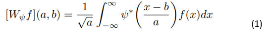
One can note this transform similarly models the fast Fourier transform (they function very similarly). The function transforms the signal f (x) using the complex conjugate of the particular wavelet ψ by taking a finite or infinite superposition between the two. The wavelet transform actually functions very similarly to that of a convolution, but instead the kernel is actually the wavelet. Similar to a convolution, wavelets can weed out specific features of a signal. In particular, the wavelets we used were capable of weeding out horizontal, vertical, and diagonal detail (Figure 1).

Figure 1: Example of different filters applied to an image through wavelet transformations.
An avid reader might wonder the difference between the wavelet transform and the Fourier transform. Both decompose the signal into their respective sinusoidal waves uncovering the frequencies, yet the Fourier transform fails to account for the time at which each sinusoidal wave is occurring at-the Wavelet transform uncovers both time and frequency domains [3].
Applications
In a more general sense, wavelet transform has applications in the fields of data and image compression, most notably in the JGP 2000 format. For example, data with abnormal variation and spikes like audio files is better compressed with wavelet transforms while data with periodic variations are better compressed with other methods such as the Fourier transform [4].
Wavelet analysis has improved the accuracy of image classification models in a different number of ways. Due to the variability of wavelets in both the frequency and time domain, wavelet functions have been used as activation functions or replacing pooling layers with wavelet transforms [5]. In our project, we simply use wavelets as a pre-processing technique while leaving many of the standard machine learning techniques unchanged.
Materials and Methods
Data gathering and preprocessing
We gathered data from the mira best batched dataset, a dataset consisting of 1256 images of radio-loud AGNs from two sky surveys: FIRST and NVSS [6]. FIRST or Faint Images of the Radio Sky at Twenty-cm was last updated in 2011 on the NRAO’s Very Large Array, an influential astronomical radio observatory in New Mexico [7,8]. It largely centered on the North and South Galactic Caps, and in the years since, it has become one of the most used surveys in radio galaxy classification tasks, forming the basis of much of the research being done in the area [9-11]. NVSS on the other hand, another survey done on the VLA, covers the sky over a negative forty-degree declination [12]. Both surveys are publicly available through FTP and Mira Best is available on Zenodo (Figure 2).

Figure 2: Illustration of mira best dataset.
Using a virtual telescope, the mira best dataset collected images from both surveys classified by FRI and FRII-type galaxies. We selected Mira Best based on a variety of factors: Size, ease of use, and image quality. Additionally, as the dataset was created to help train models in the classifying of radio galaxies and had preset data loading tools that allowed for compiling AGNs into train and test sets, so its results can be readily achieved using simple PyTorch code (as shown with its many implementations) [13].
We started by conducting an exploratory data analysis, largely looking at the distribution of image labels and ensuring that the dataset was not too unbalanced for the classification task we had in mind. We found it to have roughly 40% FRI and 60% FRII, and after concluding that the data required no other preprocessing or image restructuring, we compiled the images into the dataset’s provided train and test sets a roughly 70% to 30% split.
Another dataset we looked into was radio galaxy net a dataset with both radio and infrared channels [14]. We found its intended purpose of automated detection rather than classification to be beyond our goals of utilizing wavelet analysis.
However, as the dataset is well furnished with annotations, and contains even more galaxies (4,155 across 2,800 images), it could have a bearing on a future work’s dataset selection.
Model architecture
Prior research has proven convolutional neural networks to have significant promise in the field of computer vision for three main reasons [15].
• High accuracies on image classification tasks.
• Les computationally expensive compared to other types of neural networks and other machine learning algorithms.
• The use of convolutional layers in reducing dimensionality without losing information.
Furthermore, a significant level of research has already been done on the classification of stellar bodies and specifically, radio galaxies with ConvNets [13-16]. For those reasons, CNN was our model of choice (Figure 3).

Figure 3: Model architecture.
After creating a baseline model, a standard PyTorch Convolutional Neural Network with a total of 3,752 neurons, consisting of 3 convolutional layers, 3 pooling layers, and a single flattening layer, we trained the model. It took in gray-scale images of resolution 150 by 150 pixels.
As mentioned before, the convolutional layers can isolate single features (similar to how wavelet analysis will be applied later). Following it are the max pooling layers which reduce spatiality and tend to help mitigate overfitting.
The first convolutional layer takes in images of size 150 × 150, with a kernel size of 3, an output size of 3, and an input channel of 1. Afterward, the result is passed through a max pooling layer with a ReLU activation function that selects the maximum between 0 and its input. The same process is repeated twice more, first with a convolutional layer of kernel size 3 × 3, 3 output channels, and 3 input channels and second with a layer of the same kernel and input sizes but with 6 output channels instead of 3 (the ReLU max pooling layers after the convolutional are identical). Finally, the image is flattened and put through a fully connected layer with an output channel of 2. After that, the model was then given a cross-entropy loss function and the Adam optimizer with a learning rate of 0.01 [17].
Part of the reason behind our decision to create a base model with so few layers was a prediction that the model would over fit. To combat that issue without lowering any resolution of images that could compromise important astronomical features we simplified the model and reduced the number of neurons.
Hyper parameter optimization
After logging the results of the benchmark model (using Matplotlib and an epoch-based graphing system) and then analyzing both the accuracies and loss for the training and validation, we concluded that the model was overfitting [18].
Because of this unsatisfactory validation accuracy, we began to optimize hyperparameters hoping to find the right balance between the number of neurons and validation accuracy. So, to correct the overfitting, we started by changing the number of convolutional layers and dropout layers, lowering the number of neurons, changing activation functions, and playing with the learning rate.
As early as epoch 5 the validation loss (pictured in red) began to spike upwards, illustrating a drop in loss that continued to worsen as the model continued to train. In contrast, the training loss and accuracy point to the model’s performance on the training set being highly effective. In fact, logs of the model’s results after 20 epochs have shown training accuracy to reach as high as 90% (Figure 4).

Figure 4: Optimized baseline model’s results on the 20th epoch.
Even with optimized hyper parameters, our validation accuracy only increased minimally, by 5%. As a result, we began to seek other methods of combating overfitting, other methods that found the right trade-off between training accuracy and validation accuracy without compromising on model resolution or adding or removing images from the dataset.
Wavelet analysis
Referring back to the wavelet transform, we began by inputting each image as our f (x). The wavelet transform has the capacity to be modified for higher dimensional signals like images. With each signal (or image), we applied four different wavelets ψ that acted as filters for specific features: approximation, horizontal, vertical, and diagonal. Approximation compressed the image quality, horizontal isolated horizontal details, vertical isolated vertical details, and diagonal isolated diagonal details. We also created a “combined” details input, stacking each of the filters together into one super-image. These functions were provided by the PyWavelets library (Figure 5).

Figure 5: Example of wavelet analysis on a specific AGN.
Model training
Using the same hyper parameter-optimized CNN architecture, we created five training loops for each of the details. Each ran for twenty epochs, which we found to be sufficient to view any overfitting in a model (Figure 6).

Figure 6: Comparison of model train on unaltered images and model trained on vertical wavelet images.
Then while iterating through the batches for both the train and test sets, we started by isolating the different details using the biorthogonal bior1.3 families. Afterward, we began updating the loss and step functions. Additionally, we updated a variable that tallied the number of correct predictions, which we used to graph and log the results for both losses and both accuracies every five epochs (Table 1).
| Model | Accuracy (%) | Loss | ||
| Train | Validation | Train | Validation | |
| Baseline | 79.8 | 74.03 | 0.4377 | 0.627 |
| Approximation | 77.2 | 67.53 | 0.4654 | 0.5588 |
| Horizontal | 79.08 | 71.43 | 0.4506 | 0.5255 |
| Diagonal | 79.51 | 72.73 | 0.4397 | 0.5224 |
| Combined | 77.63 | 68.83 | 0.45 | 0.5843 |
| Vertical | 77.49 | 81.82 | 0.5153 | 0.5054 |
Table 1: Comparison of model accuracies and losses. The model trained on vertical wavelets achieved better performance compared to other models with respect to accuracy, loss, and overfitting.
Results and Discussion
Overfitting
As shown in the graph of the results for original images, the model started overfitting on epoch 6. On the other hand, our best-performing model, the CNN trained on vertical details, takes 30 epochs to over fit. Even then, the overfitting we observed is a much smaller increase in the validation loss compared to the much larger validation loss spikes of the original images.
Going beyond the vertical wavelet-trained model, and looking at the others, it seems like they all perform better with overfitting. Their validation loss is much more stable even though they do receive spikes, their occurrence is less frequent and much less drastic.
Accuracy
When we used hyperparameter optimization, the model got better at predicting new data but at a cost of overall accuracy We know that when loss decreases, the “real” accuracy is always going to increase, on the other side when loss increases like when the original model starts overfitting, the “real” accuracy starts decreasing even though the accuracy shown on the graph seems to increase.
Using this knowledge, we estimate the “real” original model accuracy to be 74.03%. For the model trained on vertical details, we estimate a validation accuracy of 81.82%, an increase of over 10.52%.
Future work
The success of wavelet analysis as a pre-processor for the machine learning model is evidence for its usage in the classification of other non-galactic images. A future application of wavelet analysis could reveal underlying features of different images. For example, if a certain RR Lyrae underwent a physical process that enunciated a diagonal feature, wavelet analysis could distinguish that well enough for the machine learning model to recognize. In regards to the methodology, we may look to try different wavelets that will filter different detail and note the changes in accuracy of those. In regards to our model, we believe that pre-trained models will fare better compared to the primitive models we used. Additionally, it should be possible to develop algorithms that could isolate different details such as a circular detail that detects a "curl" of a signal and filters those details out. A larger range of filters encapsulates more possibilities of certain predictors that may influence the classification process. In future runs of this experiments, different wavelets and pre-trained models would provide more insight into the predictability of certain astronomical bodies.
Conclusion
Even though some of the models did not get extreme increases in accuracy over the originals, every single one of them outperformed the model’s tendencies to over fit. Additionally, it appears applying wavelet transformations as a pre-processing filter reduced model overfitting In the future, wavelet transformations could be used to identify which features could be better indicators of certain galaxies For our dataset, vertical features were the best indicators in classifying galaxies from the FIRST sky survey suggesting theory could be developed around the fact that vertical details may be a In general, wavelets are extendable to any astronomical image; details that identify certain celestial bodies can be identified through wavelets. By understanding the relevant details of celestial bodies, it will also help develop astrophysics theory explaining the significance of these features. As wavelets are a relatively novel idea in signal processing, more research and programming can be done to improve the model of wavelet transforms, further expanding their usages in image classification and pre-processing.
References
- Krawczyk B (2016) Learning from imbalanced data: Open challenges and future directions. Prog Artif Intell 5: 221-232.
- Valens C (1999) A really friendly guide to wavelets.
- Yagle AE, Kwak BJ (1996) An introduction to wavelets.
- Selesnick IW (2007) Wavelet transforms-a quick study. Physics Today magazine.
- Wang L, Sun Y (2022) Image classification using convolutional neural network with wavelet domain inputs. IET Image Process 16: 2037-2048.
- Porter FA, Scaife AM (2023) MiraBest: a data set of morphologically classified radio galaxies for machine learning. RAS Tech Instr 2: 293-306.
- Becker RH, White RL, Helfand DJ (1995) The FIRST survey: faint images of the radio sky at twenty centimeters. Astron J 450: 559.
- Nair PB, Abraham RG (2010) A catalog of detailed visual morphological classifications for 14,034 galaxies in the sloan digital sky survey. Astrophys J Suppl Ser 186: 427.
- Aniyan AK, Thorat K (2017) Classifying radio galaxies with the convolutional neural network. Astrophys J Suppl Ser 230: 20.
- Slijepcevic IV, Scaife AM, Walmsley M, Bowles M, Wong OI, et al. (2024) Radio galaxy zoo: towards building the first multipurpose foundation model for radio astronomy with self-supervised learning. RAS Tech Instr 3: 19-32.
- Condon JJ, Cotton WD, Greisen EW, Yin QF, Perley RA, et al. (1998) The NRAO VLA sky survey. Astron J 115: 1693.
- Mohan D, Scaife A (2023) Mcmc to address model misspecification in deep learning classification of radio galaxies.
- Gupta N, Hayder Z, Norris RP, Huynh M, Petersson L (2024) Radio Galaxy NET: Dataset and novel computer vision algorithms for the detection of extended radio galaxies and infrared hosts. Publ Astron Soc Aust 41: e001.
- Lang N (2023) Breaking down convolutional neural networks: Understanding the magic behind image recognition.
- Tolley E (2024) Wavelet scattering networks for identifying radio galaxy morphologies. arXiv.
- Kingma DP, Ba J (2017) Adam: a method for stochastic optimization (2014). arXiv preprint.
- Lang N (2021) Breaking down Convolutional Neural Networks: Understanding the Magic behind Image Recognition. Towards Data Science.
- Lee G, Gommers R, Waselewski F, Wohlfahrt K, O'Leary A, et al. (2019) PyWavelets: A Python package for wavelet analysis. J Open Source Softw 4: 1237.