Spanish
  Chinese
  Russian
  German
  French
  Japanese
  Portuguese
  Hindi
Hindi Research Article, J Phys Res Appl Vol: 10 Issue: 8
Simulation of Second Order Linear Ordinary Differential Equations Using Quantum Annealing
Ahmed Selim Marzouki*
Department of physics , University of Tunis El-Manar, Faculty of sciences of Tunis, 1080 Tunis, Tunisia
- *Corresponding Author:
- Ahmed Selim Marzouki
Department of physics ,
University of Tunis El-Manar,
Faculty of sciences of Tunis,
1080 Tunis,
Tunisia,
Tel: 93831584;
E-mail: ahmed.selimphy@gmail.com
Received date: August, 19, 2021; Accepted date: November 15, 2021; Published date: November 25, 2021
Citation: Marzouki AS (2021) Simulation of Second Order Linear Ordinary Differential Equations Using Quantum Annealing. J Phys Res Appl 10: 8.
Abstract
We propose a quadratic unconstrained binary optimization (QUBO) formulation of a class of non-autonomous second order differential equations. The QUBO is tested with certain examples of ordinary differential equations (ODE’s) using D- Wave Quantum annealing system.
Keywords: QUBO, Adiabatic Quantum Computation
Introduction
In 1981, Richard Feynman delivered a keynote speech in the first conference on “physics and computation” held at MIT. In the speech, entitled “simulating physics with computers”, Feynman asked if physics can be simulated by a classical universal computer. He answered the question with a clear “no”. He concluded, “Nature isn’t classical, and if you want to make a simulation of Nature, you’d better make it quantum mechanical, and by golly it’s a wonderful problem, because it doesn’t look so easy.” Following Feynman’s idea, we propose to simulate some classical laws of nature using a quantum system. For that we use the Quantum Annealing (QA) method which falls under the umbrella of adiabatic quantum computation which is an alternative to the more familiar gate model of quantum computation. In the last years, QA has attracted attention as an optimization method for combinatorial problems due to its use of the famous quantum tunneling property of quantum mechanics hoping to achieve better optimal solutions for many large engineering problems. In order to employ a quantum annealing simulation, it is important to reformulate an optimization problem in the quadratic unconstrained binary optimization (QUBO) form. In the following section we present a brief overview of the quantum annealing idea.
BACKGROUND
Adiabatic Quantum Computation (AQC) was introduced by Farhi et al [1], as an alternative to circuit model quantum computing. AQC makes use of the adiabatic theorem to solve a given computation in the following way: One designs the solution of the computation to be encoded as an Eigen state (it is common to choose the Eigen state to be the ground state) of a final Hamiltonian H (tf inal) called the problem Hamiltonian.
In order to reach such solution we use a time dependent Hamiltonian H (t) for which the ground state of the initial Hamiltonian H (tinitial) is well known and easily prepared. We evolve the initial Hamiltonian adiabatically until it reaches H (tf inal), we can stay in the ground state the entire time, and thereby find the solution to our problem.
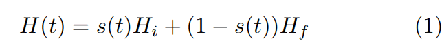
Where s (t) is an adiabatic evolution path: a function that decreases from 1 to 0 as t: 0 → tf, for some elapsed time tf. However, theoretical obstacles to adiabatic quantum computing make the practical implementation of an AQC algorithm harder to realize. Quantum annealing is a method for solving a class of optimization problems known as QUBO problems. We are given an objective function f: {0, 1} n → R x 7→ f(x) The function f assigns a cost to each configuration x and we are interested in determining the configuration that yields the minimum cost, f can be represented by a final Hamiltonian HF , with costs f(x) on the diagonal and zeros elsewhere. The algorithm starts at an initial state |ψi of HF (in general, |ψi is chosen to be a superposition of basis states as this will speed up the search making multiple computation at the same time) .Quantum systems can tunnel to other states without the need to go uphill, this will save us from some unnecessary iterations that classical methods cannot avoid. A disordering Hamiltonian HD is introduced in order to be able to control the tunneling probability in a way to favor better local minima This creates a new time-dependent Hamiltonian whose ground state will correspond to the optimal(or close to optimal) configuration f.
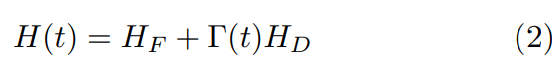
At first, the controlling coefficient Γ is set to a high value allowing the system to explore and wander around the landscape.
As time goes by, Γ (t) is decreased according to a specified schedule favouring moves towards low cost values of the objective function. At the end, the quantum system will converge towards the global minimum (or very close to the global minimum) energy of HF.
Some differences between AQC and QA are worth emphasizing (see [2]): In AQC, one derives a bound on the probability of finishing in ground state assuming the system starts in ground state. However, In QA, one analyzes the probability of converging to the ground state solution when starting from an arbitrary superposition state.
To solve a QUBO problem on a quantum annealed, the problem Hamiltonian has to be in the Ising form:
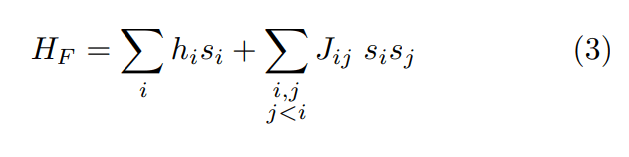
where si , sj ∈ {−1, 1} is a spin variable for the i-th spin, Jij ∈ R the interaction term between spin i and spin j, and hi ∈ R an external field interacting with spin i. It is easy to convert the spin variables to conventional binary variables xi ∈ {0, 1}, transforming the ising form to a QUBO form:
In the next section we describe the QUBO formulation of a certain class of ordinary differential equations.
Ordinary Differential Equations
Qubo Formulation
We consider the following class of non-autonomous second order ODE:
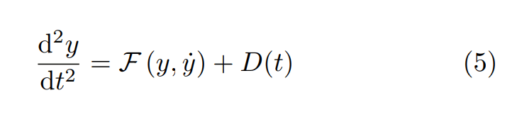
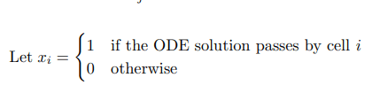
Where F is a polynomial of a degree at most two and D (t) represents a driven term . To formulate equation 5 as an optimization problem, we discretize time and space as shown in the image below:

Figure 1: Discretization of space and time coordinates.
Where Δt is the time increment, yi represents the y-value corresponding to cell i and Cj is the column of spatial cells at time tj.
Then we can write y (tj and ˙y (tj ) in terms of the binary variables xi ’s as follows:
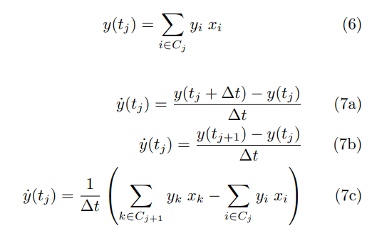
Where Cj is the j-th column of spatial cells associated with time tj, similarly, we can write ¨y as
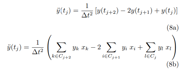
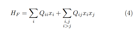
Equation 5 can be seen as an optimization problem of the form:
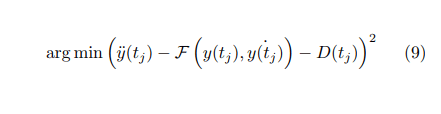
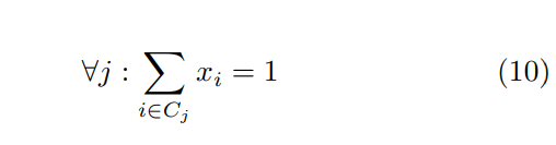
Constraint Formulation For every time slice tj, the solution y(tj ) can only be in exactly one cell of Cj , this statement can be stated as follows :
Constraint 10 can be realized as the following minimization problem:
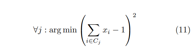
The QUBO for the non-autonomous ODE in 5 can therefore be written as:
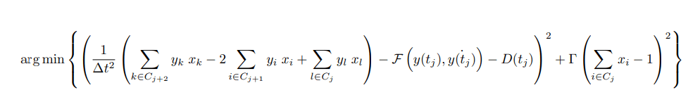
With Γ a penalty constant. In the next section we benchmark this result against some examples of ODE’s of type 5
Numerical Tests
To validate the developed QUBO, different examples of ODE are considered:
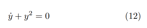
Solution to 12 is of the form y(t) = 1 t 2 . We make a python code and run the corresponding QUBO for 12 on the D-Wave Advantage system. Results of the simulation are depicted below.

Figure 2: Optimal configuration returned by the quantum annealed for the QUBO of equation 12: yellow cells are cells where xi = 1 and purple cells corresponds to xi = 0.
We fix the initial condition y(t = 1) = y281, this corresponds to the left upper corner being yellow We have obtained the behaviour of 1 t 2 function as expected from a solution of 12.
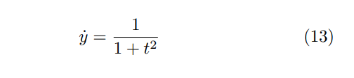

Figure 3: Optimal configuration returned by the quantum annealed for the QUBO of equation 13: yellow cells are boxes where xi = 1 and purple cells corresponds to xi = 0 we obtain the behaviour of arc tangent function which is expected from a solution to equation 13.
C) Finally, we consider the ODE describing the harmonic oscillator motion in the case of simple motion and damped motion. 1) Simple harmonic motion
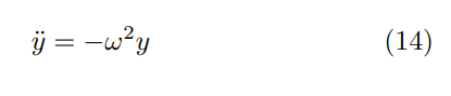
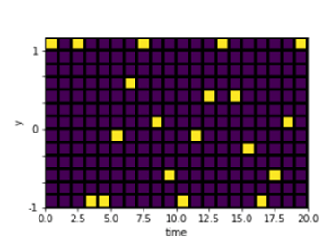
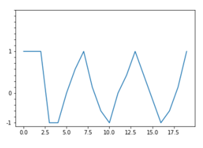
ω = 1, initial velocity v0 = 3 (b) connected points of graph a
The returned optimal configuration shows a cosine like behavior, this is in line with solutions to 14. 2) Damped harmonic motion
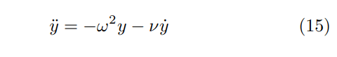
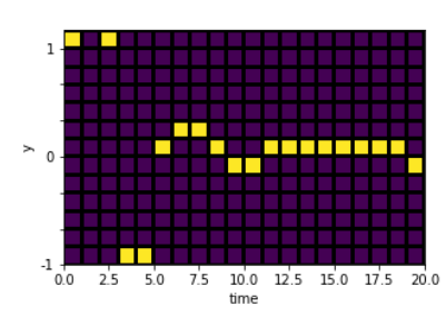
ω = 1, initial velocity v0 = 3, ν = 1.5
(b) Connected points of graph a
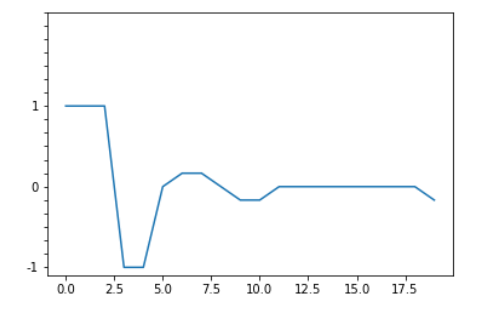
Indeed we have obtained the expected behaviour for a damped oscillator with ν 2 < ω.
Conclusion
We have provided a new way to solve a class of non-autonomous ordinary differential equations using quantum annealing. The strategy we have used to formulate the QUBO is a new one and may be applied to further problems.
Declaration of Competing Interest
The author declares that there are no known competing financial interests or personal relationships that could have appeared to influence the work reported in this paper.