Spanish
  Chinese
  Russian
  German
  French
  Japanese
  Portuguese
  Hindi
Hindi Review Article, J Health Inform Manag Vol: 1 Issue: 2
A Novel Method for Multiple Sequence Alignment Using Morphing Techniques
Quoc-Nam Tran* and Mike Wallinga
Department of Computer Science, Southeastern Louisiana University, USA
*Corresponding Author : Quoc-Nam Tran
Department of Computer Science, Southeastern Louisiana University, USA
Tel: 985-549-2189
E-mail: Qnam.Tran@gmail.com
Received: December 04, 2017 Accepted: December 12, 2017 Published: December 17, 2017
Citation: Tran Q, Wallinga M (2017) A Novel Method for Multiple Sequence Alignment Using Morphing Techniques. J Health Inform Manag 1:2.
Abstract
We review a novel computational method for Multiple Sequence Alignment (MSA), a fundamental problem in computational biology. In contrast to other known approaches, our method searches for an optimal alignment - structurally and evolutionarily by inserting or deleting gaps from a set of initial candidates in an efficient manner. Our method called a Universal Partitioning Search (UPS) approach for MSA uses graphical morphism to guarantee that the scores of the alignment candidates are always improved after each particle swarm optimization iteration.
Keywords: Multiple sequence alignment; Bioinformatics; Morphing; Particle swamp optimization
Introduction
Finding an optimal multiple sequence alignment (MSA) of three or more nucleic acid or amino acid sequences is a fundamental problem of bioinformatics with a large number of publications and citations over the last 30 years. Given a set of sequences, an optimal MSA identifies homologous characters, which have common ancestry. The resulting MSA is used for many downstream applications in medical and health informatics such as constructing phylogenetic trees, finding protein families, predicting secondary and tertiary structure of new sequences, and demonstrating the homology between new sequences and existing families.
Unfortunately, techniques that work well for pairwise alignment often become too computationally expensive when they are applied to multiple sequence alignment due the extremely large size of the search space. In fact, it is common for multiple sequence alignment problems to become computationally intractable. This is because multiple sequence alignment is a combinatorial problem, and as the number or size of the sequences in the problem set increases, the computational time required to perform an alignment increases exponentially. That is, for n sequences of length l, computing the optimal alignment exactly carries a computational complexity of O(ln). Thus, dynamic programming techniques such as the Needleman-Wunsch algorithm are guaranteed to produce optimal solutions to multiple sequence alignment problems, but are generally impractical for all but the smallest examples. Wang and Jiang demonstrated multiple sequence alignment using the sum-of-pairs heuristic to be NP-complete [1]. As a result, most currently-employed multiple sequence alignment algorithms are based on heuristics and must settle for providing a quasi-optimal alignment.
In this editorial article, we will summarize the previous works on MSA. We then provide the details of some recent computational methods for quasi-optimal multiple sequence alignments. Finally, we will discuss some possible approaches for future works.
The Sequence Alignment Problem
Sequence alignment is the process of arranging primary sequences of DNA, RNA, or protein to identify regions of similarity in order to discover functional, structural, or evolutionary relationships between the sequences [2]. These discoveries can result in the construction of phylogenetic trees, the discovery of new protein families, the prediction of secondary or tertiary structures of new sequences, and the demonstration of homology between existing families and the newly discovered sequences [3].
The general goal of sequence alignment is to find an optimum match between the sequences being investigated. This is actually a case of text manipulation, as these sequences are represented as strings over a given alphabet. For example, a DNA sequence is represented as a string drawing from an alphabet of four characters (A, C, G, and T), representing the four nucleotides. Similarly, a protein sequence is represented in the same way, but drawing from an alphabet of 20 different symbols, each representing a unique amino acid [1]. In this context, the goal of alignment is to arrange these strings so that they are vertically aligned in the optimal way to highlight similarities and differences [4]. Blank spaces, or gaps, are inserted into the strings at strategic locations so that all of the sequences are extended to the same length and the symbols in each string match vertically with the corresponding symbols in the other strings as often as possible. The optimum match is defined as the largest number of symbols from one sequence that can be match with those of another sequence while allowing for all possible gaps [5].
There are two main approaches to sequence alignment: global alignment is concerned with the best alignment of the sequences as a whole, and local alignment detects and aligns similarities in smaller "neighborhoods" [6]. The Smith-Waterman algorithm [7] is a primary example of a best local alignment algorithm, while the Needleman- Wunsch algorithm [5] is the most popular global alignment algorithm.
Regardless of which approach is used, a similarity measure is needed to quantify how well the sequences match in a given alignment, and these scores are compared to determine an optimal alignment [2]. Any similarity measure must account for changes in the sequences that are due to insertion, deletion, or mutation through evolutionary processes. This is usually done by the insertion of gaps within the sequences, presuming the presence of a gap leads to a higher number of symbol matches and thus a higher similarity score. To offset the higher score obtained through the insertion of gaps, and to prevent the introduction of an excessive number of gaps in a sequence, the similarity measure must also introduce a gap insertion penalty. Typically, two penalty values are used, one for introducing a new gap into a sequence, and one for extending an existing gap. The scoring also relies on a substitution matrix, typically from the PAM or BLOSUM families, such as PAM250 or BLOSUM62, which assigns a score to each possible amino acid substitution, with higher values assigned to symbol mutations that are more likely to naturally occur [3]. A primary example of a metric used to evaluate the quality of the alignment is the sum of pairs score (SP). Given a set of n sequences, the sum-of-pairs score is the sum of all of the corresponding pairwise alignment costs from the chosen matrix [8]. Since a naive sum-of-pairs approach treats all pairwise alignments equally, even those that are redundant or highly correlated, a weighted-sum-of-pair score is commonly used [9]. In any case, the goal is to maximize the number of matching base pairs and minimize the costs of gap penalty by deleting and inserting gaps among the sequences.
The primary disadvantage of similarity measures like weighted-sum-of-pairs is the use of general substitution matrices. These matrices generally have been formed via statistical analysis of a large number of sample alignments, but may not be adapted to the specific set of sequences being aligned for a given problem. An alternative is to use a Hidden Markov Model approach, in which sequences are used to generate statistical models to create operation sequences of gap insertions and deletions. Unlike the standard substitution matrices, the model can be developed and trained based on the characteristics of the sequences to be aligned. Given a trained model, the sequences of interest are aligned to the model in succession, producing in a multiple sequence alignment [10]. Unfortunately, there isn’t a known deterministic algorithm that can successfully guarantee an optimally trained Hidden Markov Models within a reasonable time limit. Some algorithms, such as the forward-backward algorithm (also known as the BW algorithm) by Baum and Welch uses statistical approximations to determine a suitable Hidden Markov Model. Some stochastic approaches have been tried, but generally only for smaller Hidden Markov Models (10 states or less) [11].
Progressive Methods For Multiple Sequence Alignment
Since dynamic programming techniques such as the Needleman- Wunsch algorithm are guaranteed to produce optimal solutions to multiple sequence alignment problems, but are generally impractical for all but the smallest examples, most currently-employed multiple sequence alignment algorithms are based on heuristics and must settle for providing a quasi-optimal alignment [4]. The most common heuristic method today is the progressive alignment technique. Progressive alignment requires initial guesses about the relationships between sequences in the set, and uses those guesses to build a guide tree to represent those relationships. The most closely related pairs of sequences are aligned using traditional dynamic programming methods, following the guide tree to start with the most similar pair and working towards the least similar pair. At each step, two sequences are aligned, or one sequence is aligned to an existing alignment. In the latter cases, any gaps that were introduced in earlier alignments are kept when a new sequence is added to the group. These groups of pairwise alignments are iteratively aligned together, resulting in the final multiple sequence alignment [12].
Phylogenetic trees such as a guide tree are usually produced using a similarity (or difference) matrix, so the “initial guesses” required prior to building the guide tree are actually used to construct such a matrix. The matrix classifies the sequences according to their differences, which is assumed to be a proxy for the evolutionary distance between them. The two key features of any tree are the branching order (called the topology) and the branch lengths, which should be proportional to the evolutionary distances between species. The trees that account for today’s extant species using the smallest number of historical genetic events are considered the best, so any tree-building algorithm will favour scores of high similarity (and thus, low difference) [13].
Hogeweg and Hesper’s research, published in 1984, was primarily concerned with the construction of phylogenetic trees, but also proved foundational in multiple sequence alignment. Computational tree-building methods based on molecular sequence data required a set of aligned sequences as input, which in turn required a prior assessment of the sequences’ similarity. At this point in time, there was no practical method for obtaining a multiple alignment; the computational requirements for pairwise algorithms such as Needleman- Wunsch were too much for the computers at the time to do anything beyond two sequences. So, the set of sequences was often aligned by hand using guidelines. Hogeweg and Hesper’s technique sought to improve that situation by taking advantage of pairwise alignment iteratively. Their algorithm took a set of N unaligned sequences as input and created a set of pairwise alignments and a resulting NxN similarity matrix. This similarity matrix was used to create an initial tree, and then the sequences were pairwise aligned again, this time following the branches of the tree. The new set of aligned sequences were used to create a new similarity matrix, which was in turn used to create a new tree. This iterative process continued until a specified termination criteria was met. The output of the process was the final tree and the corresponding multiple sequence alignment [14].
By contrast, Waterman’s consensus-based approach, published in 1986, did not work with phylogenetic trees at all, but focused solely on multiple sequence alignment. Waterman’s method addressed the same primary concern that Wilbur and Lipman’s method did for pairwise alignment. Whereas Waterman claimed that the most common techniques used for sequence analysis at the time aligned on single letters, his algorithm allowed for a fixed word size of arbitrary length k, just as Wilbur and Lipman’s context-based approach took into account longer sequence fragments. The choice of k was seemingly limited by the complexity of the chosen alphabet and the available computational power. The algorithm also used a specified word of length k, referred to as w, and a window width, W. The sequences could shift no more than W spaces in an attempt to find the consensus word w. If an exact match could not be found, the user could choose to allow a number of mismatches, d, up to a specified limit, with larger values of d receiving a worse weighting, λd , equal to (k-d)/k. The score s(w) for a given word w inside a given window W was calculated by multiplying q, or the number of sequences containing w (within a given number of allowed mismatches, d) inside W by the weight assigned to that d value, and summing across all allowed values of d. More formally, s(w) = Σdλdqw,d. Intuitively, the best consensus word, w*, was the one with the maximum score; in other words, s(w*) = max (s(w)) [15].
The following example contains three sequences using a fictitious 3-character alphabet consisting of A, B, and C:
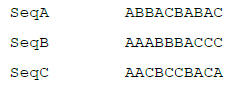
For simplicity in this example, d will be set equal to zero (so that mismatches are not allowed at all), which makes the weight λd a constant value of 1, so the scoring function reduces to a simple count of the number of sequences containing the desired word. If k is set equal to 3, there are 27 possible words, 17 of which have occurrences in the sequences:
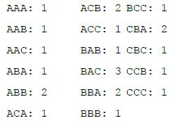
So, the best consensus word w in this example is BAC with a score 3, followed by ABB, ACB, BBA, and CBA with scores of 2 each.
However, finding a common word in all of the sequences is not the same as aligning them. To create an alignment, Waterman’s algorithm looks for a partial ordering of words; that is, a series of consensus words (w1, w2,...wn) such that the occurrence of w1 in a given sequence is to the left of the occurrence of w2 in that same sequence, without intersecting, for all sequences being aligned. The optimal alignment is one that maximizes the sum of the scores of the consensus words used, which is not necessarily the same as using the largest number of consensus words. More formally, if w1|w2 indicates that w1 and w2 can be found in nonoverlapping windows in a sequence, the goal is to find the set of words wi that satisfies S=max{Σi≥1s(wi):w1|w2|…}. Optionally, a minimum constraint s(wi)≥ c may be imposed, for some value c, to ensure that consensus words of a sufficient quality are used. For implementation purposes, S can be defined recursively as follows: Si= max {Sj+ Sj+1,i : i-W + 1≤ j ≤ i- k }, where sj+1,i is the largest scoring consensus word in the window from j + 1 to i such that all occurrences of the consensus word are to the right of the consensus words for Sj [15].
Returning to the three-sequence example, since the length of each sequence being aligned is ten, and overlapping sequences are not allowed in a partial ordering, the number of words allowed n is limited to three. Obviously, the best possible partial ordering would include three words, specifically including BAC and two words with a score of two; this is the only way the maximum score of seven could be achieved. Since the goal is to find the partial ordering with the maximum possible score, this is a good place to start. There are thirty-six possibilities for partial orderings (w1, w2, w3) involving BAC with two words with a score of two. A third of those permutations place BAC in the first position (w1), and another third place BAC in the second position (w2). None of these partial orderings are viable, since the placement of the word BAC in sequences B and C require it to be the last word in the ordering. Thus, only the twelve permutations with BAC set to w3 require further consideration (see Figure 1).

Figure 1: Three-sequence example.
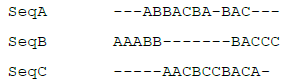
Thus, in this example, the only set of consensus words that results in the maximum score S = 7 is (w1, w2, w3) = (ABB, ACB, BAC). The resulting alignment would match the word ABB in sequences A and B, CBA in sequences A and C, and BAC in all three sequences, like so:
Waterman’s algorithm was originally coded in the C programming language, and was made available for DNA sequences only due to its smaller 4-character alphabet. Protein alignment using the usual 20-letter amino acid alphabet was limited to a maximum word length of 3 at the time. The algorithm intentionally did not include any penalty for unmatched letters due to insertions or deletions, and its result was not guaranteed to be equal to the global maximum [15]. Waterman’s algorithm was not a true progressive alignment technique, because it did not iteratively conduct pairwise alignments of two sequences in the fashion of Hogeweg and Hesper’s work. Instead, it aligned small individual words within all of the sequences, improving the alignment left-to-right as it progressively con-sidered additional consensus words.
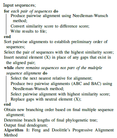
In 1987, Feng and Doolittle published a true progressive alignment method iteratively utilizing the Needleman-Wunsch pairwise alignment technique to achieve a multiple sequence alignment. Feng and Doolittle identified a consistency problem with the pairwise alignment method used in previous progressive alignment methods. That is to say, when sequence A is aligned with sequence B, gaps are inserted in particular locations. But, if either sequence A or sequence B is aligned with sequence C, the likely result is a completely different set of gaps. In general, scientists are more confident in the gap placement of the pairwise alignment of the two most similar sequences, but previous progressive alignment methods did not distinguish between levels of confidence in a given pairwise alignment. Feng and Doolittle wanted to ensure that a high-confidence gap used to align two closely related sequences was not discarded in service of improving an alignment to a more distantly related sequence. To this end, their algorithm progressively aligned sequences in pairs using the Needleman-Wunsch algorithm, starting with the most similar pair and iteratively adding the next most similar sequence, just as earlier progressive alignment techniques had done, but added an additional rule of “once a gap, always a gap.” To enforce this rule, after a pairwise alignment was completed, the newly inserted gaps were replaced with neutral characters, X. Thus, when the next sequence was added and the alignment was recalculated, necessitating new insertions and deletions, the brand new gaps would not be confused with the previous gaps (which were now X’s). The X characters were invisible to the scoring system, so that when an X was matched to any other amino acid symbol, the value was zero, not aiding the quality of the alignment, but also avoiding a new gap penalty. Once all sequences were added to the final alignment, the difference scores were calculated and the tree was constructed [13]. This process is shown in Algorithm 1.
The program was written in C and executed on a computer running the UNIX operating system. Subprograms were written and called as needed, including SCORE for conducting pairwise alignment and computing difference scores, BORD for establishing preliminary tree branching orders, BLEN for determining tree branch lengths, and DFalign for generating the multiple alignment. Feng and Doolittle reported that while their method “throttled” the pursuit of global optimization, which maximized overall similarity at the cost of removing existing gaps during the optimization process, the net gain was positive because the trees generated from their alignments appeared to more accurately agree with biological expectations [13].
The Clustal Family
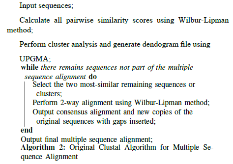
Feng and Doolittle’s progressive approach became the most popular technique for carrying out multiple sequence align-ment, and was used as the basis of the Clustal software package by Desmond Higgins and Paul Sharp [16]. In fact, Higgins and Sharp described their program as a "quick and dirty" version of Feng and Doolittle’s algorithm. It was originally implemented on an IBM AT-compatible microcomputer running at 10 MHz, with 640kb of RAM, using FORTRAN77. Much like Feng and Doolittle’s progressive alignment program, Clustal consisted of three separate subprograms that executed independently in sequence, using text files to communicate intermediate results. The first stage was the calculation of all pairwise similarity scores using Wilbur and Lipman’s algorithm to perform the pairwise alignments and produce a similarity matrix.
That matrix was then fed to the second stage of the Clustal program, which used it to derive a dendogram file using the popular UPGMA method. Dendograms can be used to represent phylogenetic trees, although in this case the output was not considered reliable enough to be used in this way. Instead, the resulting dendogram file, along with the original sequence data, was given to Clustal’s third stage, which Higgins and Sharp described as the "core" of the package. This third stage followed the order of branching in the tree to perform pairwise alignments of the most similar se-quences first, again using Wilbur and Lipman’s method. Once a pairwise alignment was complete, the consensus alignment (including gaps) for the sequence cluster was substituted into the tree, so gaps that occurred in earlier alignments were preserved if those sequences were aligned with a different sequence later, as prescribed by Feng and Doolittle. Thus, as the iteration continued, the alignments kept building upon previous consensus, and the addition of gaps was cumulative. At the end of the process, the resulting multiple sequence alignment was given as output. (See Algorithm 2.)
The second version of the program, Clustal V, was released in 1992 by Higgins, Alan Bleasby, and Rainer Fuchs [17]. It was rewritten in the C programming language. A major new feature was the ability to store and reuse old alignments (referred to as profile alignments) and align alignments with each other. Improvements to tree generation included the option to use the Neighbour-Joining method, the ability to calculate true phylogenetic trees after alignment, and the option to perform a bootstrap test to calculate confidence intervals of the tree topology [18].
A major difficulty with the progressive approach, as identified by Higgins, Julie Thompson, and Toby Gibson, is proper choice of alignment parameters. Just as with stochastic optimization methods, progressive alignment methods will produce poor results if the starting parameters are inappropriate. In this case, the alignment parameters in question are the choice of which weight matrix to use, and which two values should be used for gap penalties (one for opening a new gap and one for extending an existing gap). While a single matrix and a broad range of penalty values may work acceptably for sets of similar sequences, as the sequences become more divergent, different weight matrices may be optimal and the useful range of penalty values will narrow substantially [12].
In 1994, a new version of the software, Clustal W, made four significant improvements addressing the issue of parameter choice. First, each sequence was assigned an individual weight from the guide tree, with near-duplicate sequences receiving lower weights and more divergent sequences receiving higher weights. As part of this improvement, the guide tree creation step was changed from the UPGMA method to the Neighbor-Joining Method, which produces better estimates of the individual tree branch lengths used to derive the weights. The weights were then used as multiplication factors for scoring positions; position matches between more divergent sequences were rewarded more than matches between two nearlyidentical sequences. The second major improvement also dealt with the degree of divergence among the sequences; different substitutions matrices from the PAM and BLOSUM series were algorithmically chosen at different points in the alignment process depending on the estimated divergence of the sequences being aligned at that point. When the sequences were closely related, stricter matrices were used, and when the sequences were more divergent, more forgiving matrices were selected. The third improvement was the addition of residuespecific and position-specific gap opening penalties. As opposed to applying the same opening and extension penalties at every position, manipulating the gap opening penalties in a position-specific manner encouraged new gaps to be placed at certain positions more than others. For example, gap penalties were lowered at positions with existing gaps in one of the sequences, but increased in the areas near existing gaps. Finally, positions where gaps were added early in the iterative process were subsequently assigned reduced gap penalties, in order to encourage new gaps to be placed there rather than in brand new areas [19].
Clustal X was released in 1997. It produced the same align-ments as Clustal W, but added a graphical user interface, including pulldown menus, cut-and-paste functionality, sequence highlighting and custom coloring, and an integrated environment for performing multiple alignments, viewing results, and refining and improving the alignment as necessary. The user could interact with the results of an alignment using the mouse cursor and manually realign questionable areas [20]. The windowed interface used the NCBI Vibrant Toolkit and was made available on computers running Microsoft Windows, the Macintosh operating system, and UNIX/Linux with the X Windows System [21]. Shortly after the introduction of the windowed interface, parallelized versions and World Wide Web-based versions were made available [22].
In the late 1990s, Clustal W and Clustal X were the most widely used multiple alignment programs, but as time progressed, the need for updating and modernizing the code base became apparent. In 2007, version 2.0 of both Clustal W and Clustal X were released. The new versions were completely rewritten using the C++ language and redesigned for easier maintainability. The programs’ new object model made it easier to modify or replace the alignment algorithms in case new developments in the field necessitated it. The windowing code replaced the NCBI Vibrant Toolkit with the Qt windowing toolkit, while keeping identical functionality and still running on Windows, Macintosh, and Linux platforms. The UPGMA algorithm was reintroduced as an option for tree generation, primarily for efficiency and speed. [23].
Clustal Omega is the current version of the software package. It is another complete rewrite of the software and was first released in 2011 [24]. Two major improvements over previous versions utilize newly developed third-party packages to keep the performance and quality of results current with the state of the art. First, Clustal Omega uses an algorithm called mBed to produce the guide tree. mBed has been shown to produce just as accurate guide trees as conventional methods, while lowering the computational complexity of that step from O(N2) to O(N log N) for N sequences. Secondly, once the guide tree is in place, the alignments are computed by an implementation of HHalign, which converts sequences and intermediary profiles into Hidden Markov Models prior to alignment [25].
T-Coffee
As described in the previous section, improvements in later versions of Clustal were aimed at solving the parameter choice problem, but a second major drawback to the progressive approach is the local minimum problem. It is due to the "greedy" nature of the alignment strategy. As the most similar pairs of sequences are aligned together early in the algorithm, there is no guarantee that those pairwise alignments will place gaps in the optimal positions for the multiple sequence alignment. They will be optimal for that particular pairwise alignment, and since the best matches are being aligned first, they are assumed to be of a sufficient quality and correctness. Even so, some misalignments will occur, especially for more divergent sequences. Unfortunately, when such a misalignment occurs early on, by the nature of the algorithm, it will never be corrected later. In many cases, these misalignment errors will compound through multiple iterations. Thus, there is no guarantee that the global optimum solution for the set of sequences will be found by the progressive alignment approach [19]. Higgins, Thompson, and Gibson did not attempt any direct solutions to this problem, admitting that it is intrinsic to progressive alignment techniques. They suggested that an overall measure of multiple alignment quality could be used, and then one could find the alignment that maximized that overall measure, but such a solution was only feasible for small numbers of sequences. They posited that stochastic optimization procedures could be used in the future to this purpose [12].
This local minimum problem was addressed by Notredame’s consistency principle and the development of the COFFEE (Consistency-based Objective Function For alignment Evalu-ation) family of software tools. Originally published in 1998 by Cedric Notredame, Lisa Holm, and Desmond Higgins, the key characteristic of COFFEE is a novel objective function that measures the degree of consistency between a multiple sequence alignment and a library of pairwise alignments of the same sequences. The objective function is a global measure for evaluating an entire alignment, with a higher objective function score indicating a more biologically sound and relevant alignment [10].
The library of pairwise alignments must be built before the objective function can be used. The library is specific to a given set of sequences, so a new one must be made for each desired multiple sequence alignment. Generally speaking, given N sequences to be aligned, the library will contain at least (N2-N)/2 pairwise alignments, one for each of the possible pairings. In reality, there is no limit to the amount of redundancy that can be included in the library, so more pairwise alignments can be added as desired. Any appropriate method can be used to generate the pairwise alignments, and the amount of time required to produce the library is dependent upon the method used and increases quadratically with the number of sequences [10].
Once the library is built, evaluation of a given alignment is performed using the COFFEE objective function. Each pair of aligned residues (either two residues aligned with each other or a residue aligned with a gap) in the input alignment is compared to the contents of the library. The residues are identified by their position in the sequence, and the overall consistency score is equal to the number of pairs of residues found in the multiple alignments that are also present in the library, divided by the total number of pairs in the multiple sequence alignment, which will produce a consistency score between 0 and 1. This simplistic scoring scheme was improved by adding weighting. In the final COFFEE objective function, each pairwise alignment in the library was weighted according to the percent identity between the two aligned sequences. This ensured that the alignment of a given sequence was most influenced by its closest relatives, and that the most closely related pairs of sequences were correctly aligned in the final multiple alignment [10].
Formally, the COFFEE objective function takes as input N aligned sequences, labeled S1 through SN . Ai,j is the pairwise projection of the sequences Si and Sj, and LEN(Ai,j) is the length of this alignment. SCORE(Ai,j) is the number of aligned pairs of residues that are shared between Ai,j and the corresponding pairwise alignment in the library, and Wi,j is the weight assigned to that pairwise alignment. Then, the COFFEE score is equal to the following [10]:
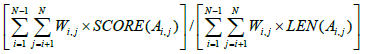 (1)
(1)
Substituting the pairwise library in place of a standard substitution matrix, the COFFEE objective function shares obvious similarities to the previously discussed weighted sum-of-pairs metric, but also has three main differences. There are no extra gap penalties assigned in the COFFEE calculation, because that information is already accounted for in the pairwise library. Second, the COFFEE score is normalized between 0 and 1. Thirdly, using the pairwise library makes the cost of the substitutions position dependent; when using a standard substitution matrix, a pair of residues will be assigned the same cost, but in COFFEE scoring the result will differ if those residues have different position indices within their sequences [10].
When evaluating the COFFEE objective function apart from the entire alignment method, Notredame demonstrated that higher scores for a sequence correlated strongly with higher average alignment accuracy. The weighting scheme and the flexibility to define the pairwise library on a case-by-case basis were the primary reasons credited for COFFEE’s positive performance [10].
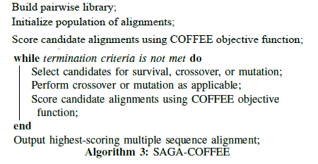
In the original COFFEE software package, the objective function was used in conjunction with the Sequence Alignment Genetic Algorithm, or SAGA, package developed by Notredame and Higgins [26]. Given an initial population of alignments, the alignments are scored using the objective function, and the result is used as a fitness measure. Based on this fitness measure, members of the population are selected for survival, crossover-based breeding, or random mutation, with the least-fit members failing to persist. The new generation is scored with the COFFEE objective function, and the process repeats. These iterations continue until the best-scoring alignment is not improved for a specific number of generations (typically 100), at which point the highest-scoring alignment in the population is selected for output [10].
Across thirteen test cases, SAGA-COFFEE was shown to outperform other methods, including Clustal W, in at least nine of them. SAGA-COFFEE performed particularly well when the sequences being aligned exhibited low levels of identity. Even though the full SAGA-COFFEE method outperformed other common approaches on average, it also proved to be extremely slow. Additionally, Notredame pointed out that it did not always produce the best alignment, and it seemed that under the right conditions, any method could do better than the others [10].
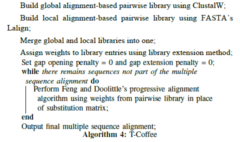
Just as new versions of Clustal brought changes and improvements to its methods, the Coffee family of software tools continued to be developed and improved. In 2000, T-Coffee (Tree-based Consistency Objective Function For alignment Evaluation) was released, which took a different approach than its predecessor. Like the original Coffee, T-Coffee uses a pairwise alignment library to guide its evaluation, but unlike the original program, it uses a more traditional progressive alignment approach instead of a genetic algorithm. While T-Coffee is still first and foremost a greedy, progressive method, it also represents a direct effort to minimize the “greediness” of the progressive alignment approach. [27].
Among progressive alignment techniques, T-Coffee’s two distinctive features are its use of heterogeneous data sources from its pairwise alignment library, and its optimization method. The former feature is similar to the original Coffee, but distinct among progressive alignment tools, and intentionally was designed to allow for a mixture of local and global pairwise alignments. During development and testing, ClustalW was used to construct the pairwise global alignments, and the Lalign program from the FASTA package was used to generate local alignments. To give priority to the most reliable pairings, weights were assigned to the alignments in the library using the same approach as the original Coffee program. When the global and local alignment sets were combined to form the library, duplicates were merged into a single entry and given a weight equal to the sum of the two original entries. Finally, the weights were adjusted using a process called library extension. First, each aligned pair was checked against the other sequences not in the pair, forming triplets. For example, given sequences A, B, C, and D, and concerning ourselves with the pairing of A and B, two triplets would be formed. ACB would be formed by combining the pairwise alignment AC with the pairwise alignment CB. Similarly, ADB would be formed using the pairwise alignments AD and DB [27].
The objective function is based on a standard progressive strategy similar to what is used in ClustalW, but integrates information from the library during each step. The progressive alignment uses a dynamic programming algorithm, but sets the gap-opening and gap-extension penalties to zero (just as gap penalties were not needed in the original genetic-algorithm-based Coffee calculation). Also as in the original Coffee, the weights from the library are used in place of the weights from a standard substitution matrix, which reduces the “greedy” effect by utilizing information that was specially generated for the current set of sequences, not only the position-dependent weighting present in the original Coffee scheme, but also the context-aware weighting produced from the library extension process described above. Once the dynamic programming algorithm has completed an alignment step, Feng and Doolittle’s “once a gap always a gap” principle is maintained; once a gap is introduced in the progressive alignment, it is never removed. The key difference here is that the placement of those gaps is better informed by data customized for this specific alignment, resulting in fewer misplaced gaps earlier in the process [27].
When tested using the BaliBase database of multiple sequence alignments, T-Coffee produced the highest average accuracy among four leading software tools (including ClustalW, Prrp, and Dialign), especially on more divergent test cases. The increased accuracy came at the expense of computational cost and running time; even when given a previously generated pairwise library, T-Coffee ran about two times slower than ClustalW [27].
Stochastic Optimization Methods For Multiple Sequence Alignment
Since multiple sequence alignment can be viewed as an optimization problem with the goal of maximizing the scoring function, it comes as no surprise that stochastic optimization and swarm intelligence techniques have emerged as a prevailing option for improving the computational cost of MSA. The two major advantages of using stochastic methods are a lower degree of complexity and greater flexibility in the objective function used for scoring, while a major disadvantage is that, by their nature, they do not guarantee optimality [10].
Several stochastic techniques have been employed with success, but drawbacks still exist. For example, simulated annealing was pursued as an alternative method by Myers and Miller and others, but has since been given consideration only as an alignment improver. It proved to be too slow to converge and was too often trapped by local optima [6].
Evolutionary algorithms such as genetic algorithms were explored, resulting in techniques such as Notredame and Higgins’ SAGA (Sequence Alignment by Genetic Algorithm) [3]. Genetic algorithms have proven to be a good alternative for finding optimal solutions for a small number of sequences, but still experience exponential growth in computational time as the number of sequences increases [6].
Novel combinations of techniques and objective functions provide reasons for optimism. A recent research project modified the objective function used by the genetic algorithm-based tool MSA-GA. MSA-GA normally uses a weighted sum-of-pairs (WSP) objective function, but weighted sum-of-pairs is known to have limitations when dealing with sequences with regions of low similarity. In 2014, Amorim, Zafalon, Neves, Pinto, Valencio, and Machado replaced the weighted sum-of-pairs objective function with Notredame’s COFFEE with promising results. The COFFEE-based implementation outperformed the WSP-based implementation in 81% of test cases with low similarity [28].
Ortuno et al. experimented with various machine learning and regression techniques to determine if they could predict the alignment quality of the several alignment tools, using 216 sequence sets from Balibase as the benchmark. Features from well-known biological databases were extracted and used to supplement and enrich the sequence information. The study used four different regression techniques: regression trees, bootstrap aggregation trees, leastsquares support vector machines (LS-SVM) and Gaussian processes. These techniques were used to estimate each alignment’s quality, with the alignment’s Baliscore value used as the benchmark. The most popular currently used alignment evaluation systems, including PAM, BLOSUM, RBLOSUM, and STRIKE, were also reference for comparison purposes. The normalized mutual information feature selection (NMIFS) procedure was used to determine which of the twenty-two selected biological features were most relevant for each model and thus worth of inclusion. The regression techniques were able to predict the quality of the alignments with a high correlation against the Baliscore values (R > 0.9), while STRIKE had a slightly worse correlation (R = 0.714) and PAM250, BLOSUM62, and GONNET had a far worse correlation with Baliscore (R < 0.21). The Gaussian and LS-SVM techniques performed the best of the four regression techniques studied, with the Gaussian processes being slightly better overall. The authors suggested that, in addition to using supplementary biological features and multiple scoring methods for alignment evaluation, these regression models could be used in the design and optimization of MSA tools, perhaps in the design of objective functions. They also suggested that traditional alignment quality scoring methods may not use enough information to provide realistic evaluations of alignments, to the detriment of the software tools that rely on them [29].
Particle Swarm Optimization For Multiple Sequence Alignment
In addition to the stochastic methods mentioned in the previous section, particle swarm optimization-based techniques for multiple sequence alignment have been utilized with positive results. However, the standard particle swarm algorithm must be modified in a few key ways to successfully adapt it to sequence alignment. First, problem-specific operators should be designed to achieve better results. Second, experimentation on parameters is often needed to obtain the most appropriate range of values. Third, problem-specific domain knowledge must be incorporated to reduce randomness and the computa-tional time required [2].
Many techniques employ a particle swarm in conjunction with another method, or in addition to an existing software tool, in order to improve the latter’s results. One of the first such techniques, published in 2003, achieved better protein sequence alignments by using a combination of particle swarm optimization and an evolutionary algorithm to train hidden Markov models (HMMs). The general approach to using hid-den Markov models to perform multiple sequence alignment, apart from using a particle swarm, is as follows: the set of states in the HMM is divided into three groups (match, insert, and delete), and the model moves between states using directed transitions with associated probabilities. The hidden Markov model uses a nondeterministic walk to generate a path of visited states and a sequence of emitted observables. The sequence of observables represents an unaligned sequence, and the goal is to find a path that yields the best alignment. The most probable state sequence path for each sequence is determined. Each match or insert state in the path emits the next symbol in the sequence, while a delete state emits a gap. Once this process has been completed for all of the sequences, they are aligned according to their common match or delete states in shared positions [11].
Before the hidden Markov model can be used, the transition and emission probabilities must be determined. The process of determining these probabilities is called "training" the hidden Markov model. No exact method for determining the probabilities has been discovered; one of the most well-known and widely-used approaches is the Baum-Welch (BW) method. Rasmussen and Krink used a particle swarm to improve the training, and seeded the swarm using initial solutions produced by the Baum-Welch algorithm and a Simulated Annealing (SA) algorithm. These two seed solutions were added to the randomly generated initial population of candidate solutions in the swarm. The candidate solutions were represented by encoding the transition and emission probabilities in the position vector of each particle, and either log-odds or sum-of-pairs was used as the objective function. New velocity vectors and particle movement were calculated as usual. Rasmussen and Krink added an evolutionary aspect to the particle swarm algorithm by including a breeding step at the end of each iteration, after the particles’ positions had been updated. Two particles bred with probability pb by performing a crossover operation on their position vectors and computing the arithmetic mean of their velocity vectors. After the breeding step, the next iteration proceeded as usual. At the conclusion of the algorithm, the global best position of the particles was considered the best hidden Markov model and the transition and emission probabilities associated with it were used to create the multiple sequence alignment. Experimental results showed that, compared to HMMs trained solely by the BW or SA algorithms, the PSO-trained version produced a final hidden Markov model with a better log-odds score and a final alignment with a better sum-ofpairs score. Despite the improvement compared to other hidden Markov model-based approaches, this algorithm was not able to match the results of Clustal W or SAGA in terms of alignment quality [11].
In 2013, Sun, Palade, Wu, and Fang proposed another technique using hidden Markov models, this time trained by a random drift particle swarm. The random drift variation is inspired by the free electron model in metal conductors placed in an external electric field, and aims to improve the particle swarm’s ability to search the problem space by modifying the velocity updating calculation. In a standard particle swarm, the position of each particle, the particle’s best value, and the global best value are all converging to a single point. A particle’s directional movement towards this single point is similar to the drift motion of an electron in metal conductors in an external electric field. The free electron model shows that, in addition to directional movement caused by the electric field, these electrons are also in a seemingly random thermal motion, resulting in the electron’s motion being expressed as a combination of a drift motion and a random motion, with velocity of V = VR +VD. The random drift particle swarm optimization algorithm uses this analogy to change the velocity calculation of the swarm particles; The random velocity VR is calculated using the distance between the particle’s position and the mean best position, mbest , multiplied by a random number from a Gaussian distribution. The drift velocity VD is calculated as usual for a simple linear of directional movement. User-specified coefficients on VR and VD control the balance between global and local search in determining the new velocity of the particle [30].
The new algorithm also introduced a diversity control measure based on each particle’s best value to help prevent premature convergence. When a particle swarm is initialized, the particles have a significant degree of diversity, but as the algorithm continues, the particles begin to converge, which lessens the diversity. Of course, this convergence is desirable for agreeing on an optimal value, but at some point, if the population diversity is too low and the global best position happens to be at a local optima, the particles will be unable to escape that premature convergence. A diversity control strategy can help prevent this. The random drift particle swarm optimization (RDPSO) algorithm calculates each particle’s Euclidean distance from the centroid of the swarm and sets a minimum distance for each iteration. If a particle’s distance crosses the threshold and is too low at a given iteration, it is altered to increase the distance until it is larger than the minimum value again. This new algorithm is referred to as random drift particle swarm optimization with diversity guided search (RDPSO-DGS). When RDPSO-DGS was used to train a HMM in much the same way as Rasmussen and Krink’s method, and compared to training by a standard particle swarm and the standalone BW algorithm, it produced the best overall performance on two benchmark data sets. The resulting HMM produced the best overall multiple sequence alignment on the same data sets, even outperforming standard MSA tools such as ClustalW. However, the RDPSO-DGS algorithm was more time-consuming [30].
Particle swarm optimization has been used in multiple sequence alignment research in other ways beyond training hidden Markov models. For example, in 2007, Rodriguez, Nino, and Alonso used a particle swarm to improve an alignment originally obtained via ClustalX. In their experiment, each particle in the swarm represented a different candidate alignment, with each particle’s coordinates representing a set of vectors specifying the positions of the gaps in each sequence. ClustalX produced an initial alignment used to seed the swarm, and other particles were derived from this seed by applying a mutation operator similar to that of a genetic algorithm. The size of the swarm was set by the user. The allowed length of a candidate alignment was given as a range, with the minimum value equal to the longest sequence to be aligned, and the maximum value defaulting to twice the length of the longest sequence. The sum-of-pairs similarity score was used as the objective function to be optimized, and the particle best and global best values were the best similarity scores obtained [3].
This algorithm proposed a variant for particle motion similar to the crossover operator from genetic algorithms. A randomly selected crossover point separated each sequence into two segments. The distance between particles was measured as a percentage of similarity; that is, the distance was measured as the number of matching gaps between two candidate alignments divided by the total number of gaps. If the distance between two particles (for example, a candidate particle and the global best) was greater than 0.5, the longer segment of the candidate particle would be replaced with the longer segment of that same sequence from the global best particle. If the distance between the particles was less than 0.5, the shorter segment would be replaced. Given the data structure used to represent each particle, this is technically achieved by removing the candidate particle’s segment’s gap from the appropriate vector, and inserting the global best particle’s segment’s gaps into that vector [3].
The algorithm was tested using seven protein families from the BALIiBASE database, and the initial alignment from ClustalX used the PAM250 substitution matrix and a gap penalty of 10. The particle swarm’s termination criterion was 10 consecutive iterations without an improvement in the global best. Under these conditions, the algorithm was able to improve the initial results obtained by ClustalX in the majority of cases [3].
In 2008, Juang and Su combined particle swarm optimization with the standard pairwise dynamic programming progressive alignment technique in an effort to escape the latter’s tendency to be trapped by local optima due to its greedy approach. In their proposed MDPPSO algorithm, dynamic programming is used to perform pairwise alignment of all sequence pairs. Next, as in standard in progressive alignment, the highest scoring sequence pair is selected, and other sequences are added to the set iteratively. In Juang and Su’s algorithm, after each dynamic programming step, particle swarm optimization was used as an improver for the intermediate alignment, to help avoid being trapped by local optima. The particle swarm algorithm modified the aligned sequence prior to the next dynamic programming iteration, and then the progressive alignment algorithm proceeded. The algorithm was tested using the BLOSUM62 scoring matrix, a gap penalty of -4, with only 5 particles and 1000 iterations in the particle swarm. They employed a randomized inertia weight value w, and used 2 for the value of both c1 and c2 in the particle swarm velocity calculation. All other parameters were assigned commonly used values with acceptable results. In their experiments with 10 different sets of proteins to be aligned, the MDPPSO algorithm produced superior alignments compared to ClustalW, T-Coffee, and other current software tools [4].
In 2009, Xu and Chen published research utilizing particle swarm optimization to perform multiple sequence alignment on its own, without the use of other tools or algorithms to initialize the swarm or conduct progressive alignment. Much like the approach taken by Rodriquez, Nino, and Alonso, a particle in the swarm represented a sequence alignment, and consisted of a set of vectors, where each vector specified the location of the gaps in a single sequence. However, in this case the swarm was initialized randomly. During initialization, in each particle, gaps were inserted at random positions into the sequences to produce an alignment. The number of gaps inserted varied, but was constrained by the maximum sequence length parameter L, which by default was set at 1.4 times the length of the longest sequence being aligned. The process was repeated until the desired number of starting alignments (particles) had been generated. Traditional sum-of-pairs scoring was used as the objective function [31].
Particle velocity and position updating were similar to that of a traditional particle swarm; each position vector in a particle was compared dimension-by-dimension against the particle’s personal best and the swarm’s global best values, and adjusted according to the standard formulas. A minor adjustment had to be added to prevent elements in the sequence from illegally swapping positions. Because the individual amino acids in a protein sequence must remain ordered, if a particle’s velocity and position calculations caused a given amino acid to move ahead of another amino acid in the sequence, the latter’s position was adjusted to be one more than the position of the former. After the particle’s velocity and position updates were finalized, if a given column in the alignment contained only gaps, that column was safely deleted from all of the sequences in the alignment at the end of the current iteration. At the end of each iteration, extra gaps were inserted into the current best alignment by a probability m to help avoid premature convergence to local optima [31].
Testing involved eight protein families from BALiBASE. Baseline alignments were created using ClustalX, using the PAM250 substitution matrix, a gap open penalty of 10, and a gap extend penalty of 0.3. The proposed algorithm performed better than ClustalX in test cases with smaller sequences and shorter sequence lengths, and similar to ClustalX otherwise. Xu and Chen recommended future research using alternative scoring methods for the objective function, speed improvements, and other initialization techniques [31].
In 2014, Gao published a paper describing a multiple sequence alignment algorithm based on particle swarm optimization with inertia weights. As with earlier research described previously in this section, each dimensional coordinate in a particle is a vector representing the positions of gaps to be inserted into the sequence. During each iteration, Gao used a random number generator to determine the new length of a particle’s candidate alignment, then used that length to determine the number of gaps that needed to be inserted into (or removed from) each sequence. Once that had been established, the velocity calculation was used to compare the current candidate to the best solutions, and determine where the new gaps should be inserted. The distinguishing characteristic of Gao’s implementation was the use of Notredame’s COFFEE as the objective function being optimized. Experimental results using a subset of the BALiBASE library produced positive results, although no substantial improvements were noted. Rather, the COFFEE-based particle swarm was viewed as an alternative, new solution for multiple sequence alignment that produced effective results [32].
Coincidentally, this same objective function substitution was also researched in 2014 by Amorim, Zafalon, Neves, Pinto, Valencio, and Machado. They worked with a genetic algorithm-based optimizer for multiple sequence alignment known as MSA-GA, and replaced the default weighted-sum-of-pairs objective function with COFFEE. Amorim found that the substitution produced better results than the standard MSA-GA settings when aligning sequences of lower similarity. This was not surprising, given COFFEE’s known strength in that situation [28].
Recent Developments For Quasi-Optimal Multiple Sequence Alignments
One of the key decisions in building a particle swarm for multiple sequence alignment involves how to encode the information in the particles. When using the swarm for a different purpose, such as to train a hidden Markov model, it is necessary for the particles to represent particular data structures. However, in the case of the swarm building or improving an alignment of sequences, a consensus seems to be forming. Based on three separate publications from three separate teams of researchers, all detailed in the previous section, the particle coordinate vectors represent the positions of the gaps in the alignment. This is both intuitive and efficient. Since the amino acids will remain the same in all of the candidate alignments, they do not need to be encoded in every particle. Storing a single copy of the actual sequences, without any gaps, saves memory space, and it is easy to construct an alignment by combining the sequences with the corresponding gap location information stored in the particle’s vectors.
The initialization of the particles in the swarm can be a crucial factor in the success of an optimization. For example, Rodriguez, Nino, and Alonso initialized their swarm by starting with an alignment from ClustalX and varying the particles using a mutation operator similar to that of a genetic algorithm, while Xu and Chen initialized their particles randomly. The UPS particle swarm in [33] borrows ideas from both of these approaches, as well as ideas found in Notredame’s COFFEE, to produce an initial swarm that is both of sufficient quality and sufficiently varied.
One of the primary advantages of using a particle swarm for function optimization is the ability to apply the same technique to many different target functions. In the case of multiple sequence alignment, previous research has focused on the same traditional metrics. Rodriguez, Nino, and Alonso and Xu and Chen’s research both used the standard sum-of-pairs scoring method as the objective function to be optimized by the swarm; Gao’s research used Notredame’s original COFFEE function. Xu and Chen specifically recommended that future research explore alternative scoring methods for the objective function, and the research in [33] attempts to expand on those previous works by introducing a new objective function named Universal Partitioning Search, or UPS. The UPS function is summarized in more detail in the following section.
Another distinguishing characteristic of a particle swarm implementation is the metric used to determine the distance between a particle’s current position and its personal best or global best position, and the application of that distance metric to the particle swarm’s standard velocity and position updating formulas. When optimizing most mathematical functions, such as the Griewank function a standard Euclidean measure of distance suffices, but multiple sequence alignment may call for more novel approaches. As discussed in the previous section, Rodriguez used a simple percentage of similarity measure to determine distance, and employed a crossover technique to move the particles. Xu attempted to keep the standard velocity and position updating formulas intact, making minor adjustments as necessary when the Euclidean calculations moved a given amino acid to an illegal position in the alignment. Gao used a random number generator to change the target lengths of candidate alignments prior to updating the particle’s velocity and position. The research in [33] uses a novel method of determining particle distance and movement, inspired by wavelet-based volume morphing techniques from the field of computer animation and image processing.
Reviewing the prior research on particle swarm optimization for multiple sequence alignment led to a few key takeaways and conclusions. First, particle swarm optimization has proven to be versatile. It has been used as a trainer, to improve the results of an alignment obtained from another method, and to produce an alignment by itself. In all cases, the results have been positive and promising, but open research questions and opportunities for further improvement remain plentiful.
Particle initialization
The particle swarm is initialized using a seed alignment, whose source can be set using a parameter value at runtime. There are currently three choices for seed values, but other options could be added easily. Two of the existing choices take a cue from Rodriguez, Nino, and Alonso, seeding the swarm using an alignment produced by either Clustal Omega or T-Coffee. When either of these options are used, the particle swarm takes on the role of an alignment improver.
The third initialization option, which is considered the default and most widely used during testing, takes inspiration from Notredame’s original COFFEE function by utilizing a library of all possible pairwise combinations of the sequences being aligned. The library was built by aligning each of the sequence pairs with the Needleman- Wunsch algorithm, using the BLOSUM62 scoring matrix and a gap penalty of -4. (These are the same settings used by Juang and Su in their research.)
Given n sequences to be aligned, each sequence is found in n-1 pairwise alignments in the library. To initialize the swarm, for a given sequence, each of its n-1 pairwise alignments is consulted, and the longest version of that sequence is selected. The seed particle, then, consists of the longest versions of each of the sequences taken from the pairwise library, padded with gaps at the end as needed to reach the length of the longest sequence.
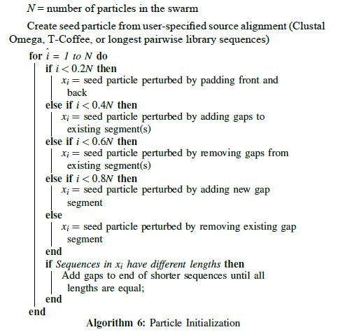
To complete initialization, in [33] each particle in the swarm must have its values perturbed so they are not identical. Rather than doing so completely randomly (as Xu and Chen reported) or using a different stochastic method (such as the genetic mutation technique used by Rodriguez, Nino, and Alonso), the particles in the swarm are divided evenly among multiple perturbation techniques, including:
1) Padding individual sequences with a random number of gaps in the front or back
2) Inserting a random number of gaps into a random gap segment in each sequence
3) Inserting a new segment of random length into each sequence at a random location
4) Removing a random number of gaps from a random gap segment in each sequence
5) Removing a randomly selected segment in each se-quence
For each of these techniques, the resulting sequences are checked for consistent lengths. If the sequence lengths in an initialized particle differ, the ends of the shorter sequences are padded with gaps to make them all the same length.
The random element of the lengthening or shortening of each candidate alignment is controlled by a user-supplied runtime parameter specifying the maximum percentage change in length. Multiple values for the parameter were tested in [33]; the best value to use varied depending upon the sequences being aligned, but 20 percent proved to be a good starting point, meaning that the initialized sequences were all between 100% and 120% of the length of the seed alignment. As a result of experimental testing, the sequences are never shorter than the seed alignment; in the case of the last two techniques, padding at the end of the sequences ensures they return to that minimum length. A more thorough investigation of the experimental results led to the default value of 20 percent. The full particle initialization routine can be seen in algorithm 6. Once initialization was complete, the candidate particles were ready to be scored using the objective function so that the initial pbest and gbest values could be determined.
The universal partitioning search optimization function
If one is not concerned with penalties associated with gap insertion, it is trivial to create a multiple sequence alignment with amino acids perfectly aligned but spaced far apart. This also increases the potential for orphans to occur in the alignment. This strategy can result in high scores under certain circumstances, but the resulting alignments are not desirable or biologically sound.
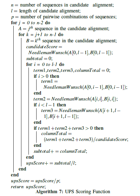
The goal of the new Universal Partitioning Search optimization function in [33] is to penalize egregious gap insertions and favor alignment candidates with large blocks of homogeneous columns. To that end, the UPS function considers not only the individual column-wise matching score between the sequences being aligned, but also the effects of that column on the quality of the alignment before and after it. An alignment candidate is split into all possible pairwise alignments, and each pair is scored individually. While traversing through each pair column-by-column, three partitions are created at each step. The first partition includes all columns in the pairwise alignment leading up to the current column. The second partition is the current column itself. The final partition includes the remaining columns from the current column to the end of the pairwise alignment.
The Needleman-Wunsch algorithm is applied to all three partitions, with the score for each partition equal to the lower-right entry in the Needleman-Wunsch scoring matrix produced for the alignment of that partition. The sum of these three scores is compared to the Needleman-Wunsch score for the pairwise alignment as a whole, yielding a subscore for the current column. The subscores of all of the columns are summed and then divided by the length of the candidate alignment, producing the average score across all of the columns for that pairwise alignment. This process is repeated for all pairwise alignments in the candidate alignment, summing all of the average scores, and ultimately dividing by the number of pairwise alignments to arrive at the overall average score for the candidate alignment as a whole. This process is shown in algorithm 7.
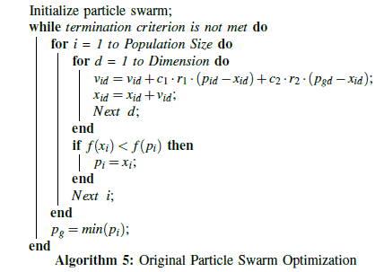
After the UPS objective function was applied to the initialized particles, it was time to iterate through the standard particle swarm optimization routine (see algorithm 5). In order to do so, a distance metric and calculations for particle velocity and movement needed to be specified (Figure 2).

Figure 2: One-Dimensional Correspondence Mapping [35].
Applying computer graphics techniques for particle distance and motion
In its first design of the UPS particle swarm in [33], the standard Hamming distance was used as the measurement between a particle’s current position and its pbest or gbest position. The Hamming distance represented the number of gap placements between the two that differed. Velocity and particle movement were based on this Hamming distance, and attempted to move a candidate particle towards the pbest or gbest values by reducing the difference in Hamming values. In the standard particle swarm velocity formula vid = vid + c1 r1 (pid-xid ) + c2.r2.(pgd-xid ), the first term is the particle’s previous velocity, and the second and third terms are the distances between the pbest and gbest , respectively. In trials where a maximum velocity value, Vmax, was used, particles tended to achieve maximum velocity very early in the program’s execution, and remained there until convergence. Unsurprisingly, convergence also tended to happen quickly, because gaps were added rapidly until they matched the number of gaps found in the best particles. This led to particles frequently becoming trapped by local optima, because they became too similar to the pbest or gbest too soon; if an early gbest value was actually a local optima, the particles would rush there too quickly and not give the algorithm a chance to find a better gbest .
A second attempt in [33] retreated from the Hamming distance approach, and tried a simpler counting method that simply counted how many gaps the particle contained in each sequence, and subtracted that value from the number of gaps in the pbest or gbest . This allowed for both positive and negative distances, with positive distances indicating that the best coordinates contained more gaps than the candidate particle, and negative distances indicating the candidate particle contained more gaps. The possibility of both positive and negative distances allowed the velocity calculation to increase or decrease from one iteration to the next, with positive velocities causing gaps to be added to the candidate particle, and negative velocities causing gaps to be removed. Unfortunately, the net effect was the opposite as the revised Hamming distance technique. As the particles approached the same number of gaps as the pbest or gbest values, their velocity’s absolute value approached zero early in the program’s execution and stayed there. This premature convergence resulted in little to no change from one iteration to the next, and did not solve the local optima tendency.
It became clear a more nuanced and sophisticated view of particle distance and movement was needed.
In the field of computer image processing, “morphing” is a technique used to create a metamorphosis from one image to another by specifying a warp that distorts the first image until it resembles the second. The technique produces a sequence of images such that the early images in the sequences more closely resemble the first source image. As the process continues, the middle image of the sequence is the average of the two source images, and the latter images increasingly resemble the second source image [34].
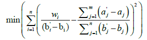
A challenge to implementing this technique is the “correspondence problem,” which involves determining which elements of the first source image should be mapped to a given element of the second source image. He, Wang, and Kaufman addressed this problem using a wavelet transform. They explained their approach first in one dimension, and then extended it to three dimensions. The one-dimensional case is of primary interest here. We begin with two one-dimensional objects, A and B, each containing multiple object segments. Without loss of generality, we define A containing m object segments and B containing n object segments, with m greater than or equal to n. Each object segment in A must be mapped to only one object segment in B, and the object segments of A should be mapped onto B as evenly as possible to minimize shape distortion. Thus, the optimal correspondence is the one that most “evenly” distributes the m segments of A onto the n segments of B by minimizing the variance using this formula [35]:
 (2)
(2)
For a given example, the second term inside the parentheses is a constant, representing the ratio between the total length of segments in A and the total length of segments in B. The individual lengths of the segments of B are also constant, and the denominator of the first term will iterate through those lengths. The values for w (the combined width of the segments from A being mapped to the current segment of B) will change depending on the correspondence mapping being considered [35]. The correspondence mapping between object segments that produces the minimum variance is considered optimal. Once it has been determined, morphing between the two objects can proceed.
This approach has been applied to particle swarm optimization for multiple sequence alignment in [33]. Each particle contains a candidate alignment, and each sequence in that candidate alignment contains segments of gaps in between the amino acids. In this way, a sequence in the candidate alignment corresponds to the object A, and the gap segments in that sequence correspond to the m segments. The second source object, B, corresponds to either the particle’s personal best (pbest) or the swarm’s global best (gbest ), and those gap segments correspond to the n segments. For each particle in the swarm, He, Wang, and Kaufman’s variance calculation and one-dimensional correspondence mapping technique are applied to the gap segments in each sequence, obtaining the optimal mapping between the gap segments in the particle’s current alignment and the gap segments in the best alignment. This is shown in algorithm 8.
The following two examples illustrate this approach. For both, assume we are given two sequences, A (containing 5 gap segments) and B (containing 3 gap segments). There are six possible correspondence mappings from A to B, listed in Table 1. Going forward, each mapping will be referred to by the number in the leftmost column.
| Mapping | B1 | B2 | B3 |
|---|---|---|---|
| 1 | Al | A2 | A3:A5 |
| 2 | Al | A2:A3 | A4:A5 |
| 3 | Al | A2:A4 | A5 |
| 4 | Al:A2 | A3 | A4:A5 |
| 5 | Al:A2 | A3:A4 | A5 |
| 6 | Al:A3 | A4 | A5 |
Table 1: Six possible correspondence mappings from A to B.
For the first example, A contains 5 gap segments and a total of 12 gaps, while B has 3 gap segments and a total of 10 gaps. The gap placements of the two segments are shown in Figure 3.

Figure 3: Sequences for Correspondence Mapping Example 1.
Applying the variance formula to this example, the second term will always be 1.2 (12 divided by10). The lengths of the segments in B (used in the denominator of the first term) are 4, 3, and 3. The values for w, the full variance calculation, and the final result for each possible mapping are presented in Table 2.
| Mapping | W1 | W2 | W3 | Variance Calculation | Result |
|---|---|---|---|---|---|
| 1 | 3 | 2 | 7 | (0.75-1.2)^2 + (0.67-1.2)^2 + (2.33-1.2)^2 | 1.77139 |
| 2 | 3 | 3 | 6 | (0.75-1.2)^2 + (1-1.2)^2 + (2-1.2)^2 | 0.8825 |
| 3 | 3 | 7 | 2 | (0.75-1.2)^2 + (2.33-1.2)^2 + (0.67-1.2)^2 | 1.77139 |
| 4 | 5 | 1 | 6 | (1.25-1.2)^2 + (0.33-1.2)^2 + (2-1.2)^2 | 1.39361 |
| 5 | 5 | 5 | 2 | (1.25-1.2)^2 + (1.67-1.2)^2 + (0.67-1.2)^2 | 0.50472 |
| 6 | 6 | 4 | 2 | (1.5-1.2)^2 + (1.33-1.2)^2 + (0.67-1.2)^2 | 0.39222 |
Table 2: Variances for each possible mapping in example 1.
The table indicates correspondence mapping #6 is the optimal one to use, which is in Figure 4.

Figure 4: Final Correspondence Mapping for Example 1.
For the second example, as before, A has 5 segments and a total of 12 gaps, and B contains three segments and a total of 10 gaps. But, the distribution of the gaps varies, as shown in Figure 5.

Figure 5: Sequences for Correspondence Mapping Example 2.
Once again, the second term of the variance calculation will always be 1.2 (12 divided by10). The lengths of the segments in B (used in the denominator of the first term) are 2, 3, and 5. The values for w, the full variance calculation, and the final result for each possible mapping are presented in Table 3.
| Mapping | W1 | W2 | W3 | Variance Calculation | Result |
|---|---|---|---|---|---|
| 1 | 2 | 6 | 4 | (1-1.2)^2 + (2-1.2)^2 + (0.8-1.2)^2 | 0.84000 |
| 2 | 2 | 7 | 3 | (1-1.2)^2 + (2.33-1.2)^2 4- (0.6-1.2)^2 | 1.68444 |
| 3 | 2 | 9 | 1 | (1-1.2)^2 + (3-1.2)^2 + (0.2-1.2)^2 | 4.28000 |
| 4 | 8 | 1 | 3 | (4-1.2)^2 + (0.33-1.2)^2 -I- (0.6-1.2)^2 | 8.95111 |
| 5 | 8 | 3 | 1 | (4-1.2)^2 + (1-1.2)^2 4- (0.2-1.2)^2 | 8.88000 |
| 6 | 9 | 2 | 1 | (4.5-1.2)^2 + (0.67-1.2)^2 + (0.2-1.2)^2 | 12.17444 |
Table 3: Variances for each possible mapping in example 2.
This suggests that correspondence mapping #1 is the optimal one to use, which is in Figure 6.

Figure 6: Final Correspondence Mapping for Example 2
Once a correspondence mapping has been established between the two sequences, it is used to move the particles from one iteration to the next. In place of the traditional PSO’s velocity and position calculations, the particle’s candidate alignment is morphed towards the pbest or gbest alignment. Traditional particle swarm optimization uses a random number generator to determine the extent that the distance between the particle’s current position and the best position(s) should influence the particle’s movement. Likewise, random number generators are used in the morphing technique to determine the extent to which the current particle’s gap segments will morph towards the gap segments in the best-scoring alignments, with smaller random numbers keeping the end result closer to the particle’s original segments, and larger random numbers pushing them towards the best segments.
For example, in the final correspondence mapping in Figure 6, sequence A’s second gap segment (in positions 7 through 12) is mapped to sequence B’s second gap segment (in positions 9 through 11). The morphing technique must determine the “velocity” of A’s segment so it can change its position; that is, how closely will it resemble B’s gap segment at the end of this iteration? Since the segment from A is starting with a length of 6 and is mapped to a segment with a length of 3, the velocity and position change of this iteration could conclude with a segment length of 3, 4, 5, or 6. In this case, a generated random number between 0 and 0.25 would imply a small velocity, and thus a small position change, keeping the segment as it is. A random number between 0.25 and 0.5 would move the particle slightly towards sequence B by reducing the segment length to 5 gaps, and a number between 0.5 and 0.75 would move it closer to sequence B by reducing the segment length to 4 gaps. A random number greater than 0.75 would imply a large velocity and fully move the particle’s position towards sequence B’s best position, so that the gap segment length is reduced to 3. More formally, the calculations for this particle movement are shown in algorithm 9.
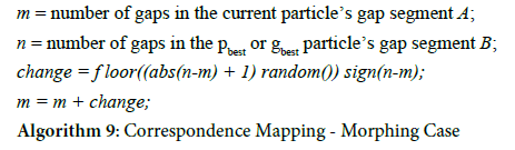
The morphing case described in the previous paragraph is the simplest possibility, in which one segment from sequence A is mapped to one segment in sequence B. It may also be the case that multiple segments from A map to a single segment in B. In this case, multiple segments must be merged into one. In figure 6, this is seen in the rightmost three segments of sequence A being mapped to the rightmost segment of sequence B. Furthermore, the three segments in sequence A collectively contain four gaps, while the single sequence in sequence B contains five. Thus, in this “merge” case, the random number generator used for the velocity must determine two separate position changes: the total number of gap segments and the total number of gaps. In this implementation, the gap segments are merged first. In the current example, a random number less than 0.33 would keep all three rightmost segments of A separate, a random number between 0.33 and 0.67 would merge the first two segments but leave the third separated, and a random number 0.67 or greater would merge all three segments into one. Once the merging is complete, the number of gaps in the merged segments would be adjusted towards the number of gaps in sequence B’s segment in the same way that was done in the morphing case. This is shown in algorithm 10.
The final possibility is a split, where a single gap segment from sequence A maps to multiple gap segments in sequence B. Due to the variance formula’s stipulation that the number of segments in A is greater than or equal to the number of segments in B, this possibility can’t be handled as-is. However, it readily occurs in the multiple sequence alignment problem; one can envision a situation where a sequence in a candidate alignment contains fewer gap segments than the global bestalignment (which likely came from a different particle). In order to move the candidate towards the global best alignment, at least one of its gap segments will need to be split into multiple segments, so that it more closely resembles the global best.
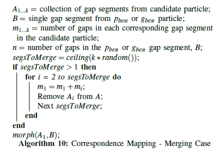
Initially, when it is discovered that B contains more segments than A, this case is handled by simply reversing the order of the correspondence mapping; rather than determining the optimal mapping from A to B, the implementation determines the optimal from B to A; that is, from the better alignment to the candidate alignment. Once the mapping has been determined, the only difference between the split case and the merge case is that the meaning of the randomly generated number is reversed; rather than smaller random values keeping the candidate closer to itself, and larger values moving it closer towards the global best, in this case the larger values will produce a new positioning that is closer to the original candidate, and smaller values will lead to a new positioning that more closely resembles the global best alignment. This is accomplished by simply calling the merging function with the order of the arguments reversed, as shown in algorithm 11.
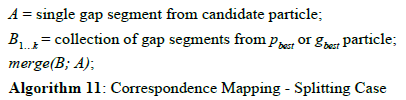
The complete process for a single particle’s candidate alignment combines the correspondence mapping and the choice between the morphing, merging, and splitting cases. This algorithm would be repeated for each particle in the swarm, during every iteration of the particle swarm optimization process.
The final consideration for adapting the correspondence mapping and morphing algorithms to replace the particle swarm’s velocity and position updating calculations involves the cognitive and social parameters, c1 and c2, shown in algorithm 5. The traditional particle swarm algorithm uses those two parameters to control the relative influence of a particle’s individual best position and the swarm’s global best position on the particle’s flight path. To accomplish the same effect, this implementation conducts three correspondence mappings for each particle in each iteration. First, the particle’s current position is morphed with the particle’s pbest, using a random number corresponding to r1 in the traditional particle swarm velocity calculation to determine the degree of the morph. Second, the particle’s current position is morphed with the swarm’s gbest, using a random number corresponding to r2 to determine the degree of the morph. Finally, these two intermediate results are morphed with each other, using the fraction c1/(c1+c2) in place of the random number. Thus, in the case that c1 and c2 are equal, the candidate’s new position will be determined equally by its movement towards pbest and gbest . If c1 is smaller than c2, gbest will carry more influence. Similarly, if c1 is greater than c2, the particle’s pbest will carry more influence. This process is shown in algorithm 13. The function called by mapping() is the mapping procedure shown in algorithm 12, which calls the morph(), merge(), and split() functions described in algorithms 9, 10, and 11, respectively, with one difference: each of those four functions would take an additional floating point parameter that would ultimately replace the calls to random() found in the morph() and merge() functions. This way, the call to random() can be initiated here when it is appropriate, or replaced with a floating point value derived from c1 and c2 when necessary.
The segment morphing technique described here contains parallels to the previous Hamming distance implementation. First, as a distance metric it is focused on the difference in the gap placements between the candidate particle and the pbest or gbest particle. Second, the use of random number generation varies the degree that the candidate particle moves towards the pbest or gbest .
However, the key advantage to the new morphing approach in [33] is that it operates at the segment level, rather than the individual gap level. The morphing calculation is more concerned with the optimal way to move the existing gap segments to become more like the gap segments found in the pbest or gbest , and less concerned with the number or position of individual gaps. As shown in the illustrated examples, the number of gaps in a given segment can increase or decrease as the candidate transitions towards the pbest or gbest , so there is no concern over a monotonic increase in the number of gaps. Thus, there is less of a “rush” to converge around an early gbest value, and being trapped by local optima is less common.
In the current implementation, the objective function indicated by f() in algorithm 13 is the UPS scoring metric described in this session. Importantly, other objective functions could be used in its place; there is no coupling between the UPS objective function and the morphing technique for distance, velocity, and movement.
Approaches for future work
MSA is a fundamental problem in computational biology. New approach for MSA uses graphical morphism to guarantee that the scores of the alignment candidates are improved in some way after each particle swarm optimization iteration. A few areas of the method can be improved such as (a) efficiently handle the monotonic increase in the number of gaps. In this rare situation, a “rush” to converge around an (b) early gbest value will have the particles trapped by local optima; and design a better objective function for optimization. Since there is no coupling between the UPS objective function and the morphing technique for distance, velocity, and movement, better objective function will definitely help to further improve the method.
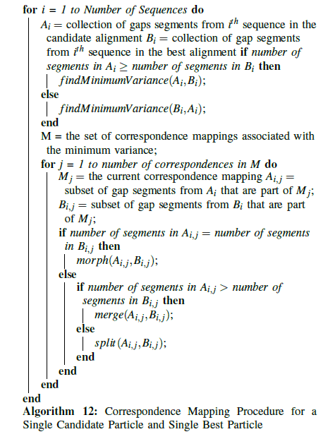
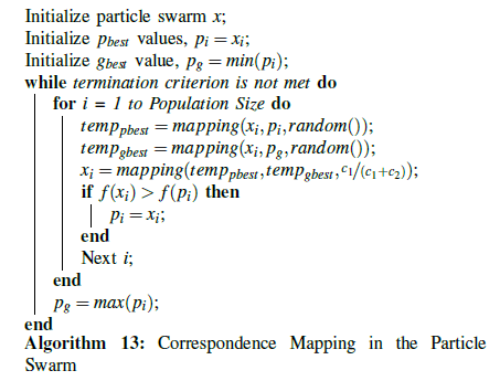
Another note is on the need of using High Performance Computing (HPC) techniques for improving the performance of PSO-based algorithms for MSA. PSO-based algorithms are inherently parallelizable. But, due to the amount of data needed for the communication between particles, using the technologies from the next generation of GPU-CPU parallelism would be more viable. GPU-based computation offers the advantages of large-scale parallelism and implementation using industry-standard libraries and tools such as NVidia’s CUDA. With significant changes to the traditional particle swarm algorithm, including replacing the velocity and distance calculations, and using a computationally complex objective scoring function, adapting the implementation for parallel execution using CUDA would undoubtedly be a challenge but would also yield impressive improvements in running time.
References
- Wang L, Jiang T (1994) On the complexity of multiple sequence alignment. J Comput Biol 1: 337-348.
- Das S, Abraham A, Konar A (2008) Swarm intelligence algorithms in bioinformatics. Stud Comput IntellS 94: 113-147.
- Rodriguez P, Nino L, Alonso O (2007) Multiple sequence alignment using swarm intelligence. Int J Comput Intel Res 3: 123-130.
- Juang WS, Su SF (2008) Multiple sequence alignment using modified dynamic programming and particle swarm optimization. J Chinese Inst Eng 31: 5-17.
- Needleman S, Wunsch C (1970) A general method applicable to the search for similarities in the amino acid sequence of two proteins. J Mol Biol 48: 443-453.
- Bucak, Uslan V (2011) Sequence alignment from the perspective of stochastic optimization - a survey. Turkish J Elec Eng Comput Sci 19: 157-173.
- Smith T, Waterman M (1981) Identification of common molecular subsequences. J Mol Biol 147: 195-197.
- Bacon DJ, Anderson WF (1986) Multiple sequence alignment. J Mol Biol 191: 153-161.
- Altschul S, Erickson B (1986) Optimal sequence alignment using affine gap costs. Bull Math Biol 48: 603-616.
- Notredame C, Holm L, Higgins D (1998) Coffee: An objective function for multiple sequence alignments. Bioinfor 14: 407-422.
- Rasmussen T, Krink T (2003) Improved hidden markov model training for multiple sequence alignment by a particle swarm optimization-evolutionary algorithm hybrid. BioSys 72: 5-17.
- Higgins DG, Thompson JD, Gibson TJ (1996) Using clustal for multiple sequence alignments. Methods Enzymol 266: 383–402.
- Feng D, Doolittle R. (1987) Progressive sequence alignment as a pre-requisite to correct phylogenetic trees. J Mol Evol 25: 351–360.
- Hogeweg P, Hesper B (1984) The alignment of sets of sequences and the construction of phyletic trees: an integrated method. J Mol Evol 20: 175–186.
- Waterman M (1986) Multiple sequence alignment by consensus. Nucleic Acids Res 14: 9095–9102.
- Higgins DG, Sharp PM (1988) Clustal: a package for performing multiple sequence alignment on a microcomputer. Gene 73: 237–244.
- Higgins DG, Bleasby AJ, Fuchs R (1992) Clustal V: improved software for multiple sequence alignment. Bioinformatics 8: 189–191.
- Higgins DG, (1994) Clustal V: Multiple Sequence Alignment of DNA and Protein Sequences. Totowa, NJ: Humana Press 307–318.
- Thompson JD, Higgins DG, Gibson TJ (1994) Clustal w: improving the sensitivity of progressive multiple sequence alignment through sequence weighting, position-specific gap penalties and weight matrix choice. Nucleic Acids Res 22: 4673–4680.
- Thompson JD, Gibson TJ, Plewniak F., Jeanmougin F, Higgins DG (1997) The clustal x windows interface: flexible strategies for multiple sequence alignment aided by quality analysis tools. Nucleic Acids Res 25: 4876–4882.
- Jeanmougin F, Thompson JD, Gouy M, Higgins DG, Gib-son TJ (1998) Multiple sequence alignment with clustal x. Trends Biochem Sci 23: 403–405.
- Chenna R, Sugawara H, Koike T, Lopez R., Gibson TJ, et al. (2003) Multiple sequence alignment with the clustal series of programs. Nucleic Acids Res 31: 3497.
- Larkin M, Blackshields G, Brown N, Chenna R., McGettigan P, et al. (2007) Clustal w and clustal x version 2.0. Bioinformatics, 23: 2947.
- Sievers F, Wilm A, Dineen D, Gibson T, Karplus K, et al. (2011) Fast, scalable generation of high-quality protein multiple sequence alignments using clustal omega. Molecular Systems Biology 7: 1–6.
- Sievers F, Higgins DG (2014) Clustal Omega, Accurate Alignment of Very Large Numbers of Sequences. Totowa, NJ: Humana Press 105–116.
- Notredame C, Higgins DG, (1996) Saga: sequence alignment by genetic algorithm. Nucleic Acids Res 24: 1515–1524.
- Notredame C, Higgins DG, Heringa J (2000) T-coffee: a novel method for fast and accurate multiple sequence alignment. J Mol Biol 302: 205–217.
- Amorim G, Zafalon L, Neves A, Pinto C, Valencio, et al. (2015) Improvements in the sensibility of msa-ga tool using coffee objective function. J Phys Conf Ser 574: 1–4.
- Ortuno F, Valenzuela O, Prieto B, Saez-Lara M, Torres C, et al. (2015) Comparing different machine learning and math-ematical regression models to evaluate multiple sequence alignments. Neurocomputing 164: 123–136.
- Sun J, Palade V, Wu X, Fang W (2013) Multiple sequence alignment with hidden markov models learned by random drift particle swarm optimization. IEEE Trans Comput Biol Bioinform 11: 243–257.
- Xu F, Chen Y, (2009) A method for multiple sequence alignment based on particle swarm optimization.Fifth International Conference on Intelligent Computing 965–973.
- Gao Y (2014) A multiple sequence alignment algorithm based on inertia weights particle swarm optimization. Journal Bionanoscience 8: 400–404.
- Tran QN , Wallinga M (2017) Ups: A new approach for multiple sequence alignment using morphing techniques. In Proceedings of the 2017 IEEE BIBM conference. IEEE 425–430.
- Beier T, Neely S (1992) Feature-based image metamorphosis. ACM SIGGRAPH Computer Graphics 26: 35–42
- He T, Wang S, KaufmanA (1994) Wavelet-based volume morphing. In Proceedings of IEEE Conference on Visualization. IEEE 85–92.