Spanish
  Chinese
  Russian
  German
  French
  Japanese
  Portuguese
  Hindi
Hindi Research Article, Res J Econ Vol: 2 Issue: 2
The Relationship between Systematic Risk, Previous Returns and Expected Stock Returns in Iranian Companies
Shaho Heidari Gandoman1* and Mohammad Rostami2
1Department of Accounting, University of Kurdistan, Iran
2Department of Accounting, Islamic Azad University, Iran
*Corresponding Author : Shaho Heidari Gandoman
Department of Accounting, Sanandaj, University of Kurdistan, Iran
Tel: +09186622083
E-mail: shahoheidari@yahoo.com
Received: December 01, 2017 Accepted: February 28, 2018 Published: March 07, 2018
Citation: Gandoman SH, Rostami M (2018) The Relationship between Systematic Risk, Previous Returns and Expected Stock Returns in Iranian Companies. Res J Econ 2:2.
Abstract
The purpose of this study was to examine the relationship between systematic risk criteria, previous return and expected return of Iranian companies. This study is a library and analytical-causal research and is based on the analysis of panel data. In this research, financial data of 105 firms accepted in Tehran Stock Exchange during the period of 2010-2015 has been investigated. The results of the research regarding the confirmation of the first hypothesis of the research showed that there is a significant and direct relationship between the systemic risk criteria and the previous returns of the firms. Also, according to the analysis done in connection with the confirmation of the second research hypothesis, we concluded that there is a significant and direct relationship between the systematic risk criteria and the expected return of the firms.
Keywords: Systematic risk; Stock Exchange; Expected return of firms; Data panel
Introduction
Large corporate executives are looking for a suitable risk-related business model and they are always trying to reduce fluctuations in profits during the fiscal year and increase stock return fluctuations in a positive direction, and control the expected return on stocks during the downturn. Controlling risk as a preventive measure reduces the intensity of the structural fluctuations of economic shocks and was first proposed by Loungani. Other researchers, such as Black, also suggested that the fundamental factor in previous returns were economic, such as the rate of economic growth. Recently, Bloom and colleagues argued that shocks created by predictions of expected stock returns would improve the business cycle and the life span of corporate business cycles.
Statement of the problem
With the expansion of business entities and diversification in production, large corporations have been created and today stock transfers and receiving stock returns are considered as one of the key issues in the economies of countries [1]. Ongoing Increase of investment in stock markets, and thus the increase of the volume of trades, requires the creation of online regulations in the economy of countries [2]. Blitz et al. [3] concluded that the two factors on the risk of the firm and the expected return on stocks in most of the capital market companies are a milestone in boosting stock exchanges [4,5]. Theoretically, investment is divided into two short- and long-term investment sectors. Regarding long-term investments, that are part of the long-term corporate goals, stock returns from firm’s risk will be very effective in relation to investment policies [6]. Regarding the main goal of this research, the researcher seeks to find out whether the systematic risk-taking criterion affects previous returns and expected returns on stocks in admitted firms is effective on Iranian firms.
Significance of the study
One of the most important financial issues in the country’s economy is the discussion of dividend fluctuations and volume of transactions and paying attention to the risk of firms in Tehran Stock Exchange. Considering the importance of the variables of the growth rate of stock returns, the volume of stock transactions, the systematic risk criteria, the company’s growth opportunities and the return on the stock market, and its impact on the volume and amount of transactions, it turns out that companies that have high risk-taking in relation to changes will experience positive or negative fluctuations in profits in their research showed that magnifying the importance of systematic risk factor regarding the fluctuations in stock returns as a factor in unblocking transactions by managers has led to attracting more investors, and this testifies to increased efficiency and high performance of companies. Also, the relationship between the factors affecting the stocks return from the company’s risk will be an important factor in boosting the capital market [6]. The attraction of investors in the capital market of our country, considering the emergence of the capital market compared to advanced countries is very important for managers. In order to reach this goal, identifying the influence ratio of factors such as fluctuations in previous stock returns and stock returns due to company risk and its impact on expected stock return can be the key to achieving the ultimate goal of companies which is maximum profitability.
Research Hypothesis
• First hypothesis: There is a meaningful relationship between the systemic risk criteria and previous company returns.
• Second hypothesis: There is a significant relationship between the systemic risk criteria and the expected returns of the companies.
The variables of this research are classified into three groups
Dependent variables
• i company’s previous returns in year t.
• Expected returns of i company in year t.
Independent variable:
• The systematic risk factor of company i in year t.
Control variables
• Size of company i in year t.
• Growth opportunities of company i in year t.
• The ratio of stock trades of company i in year t.
• The negative return of company i in year t.
• Conflict of previous returns and company risk of company i in year t.
Test of empirical Cdf fluctuations
In the test of fluctuations of empirical growth of variables, through a graph, the empirical growth of variables are shown over the years under study. Empirical growth of variables indicates the positive or negative growth rates of these variables, taking into account the amount of deviations existing. The positive or negative growth rates of dependent, independent and control variables are displayed simultaneously in a graph. One of the influential properties of this test is to identify the degree of convergence of growth variables for the final estimation of the model based on the data of panel data. The estimated graph of the empirical growth of variables is estimated by Minitab 17.1 software as follows (Figure 1):

Figure 1: Test of empirical Cdf fluctuations.
Descriptive statistics of the research variables
The descriptive statistics status of the model variables after screening and deletion of data using SPSS 20 software is presented in Table 1
| Variable | Number of Observations | Mean | Standard Deviation | Minimum Amount | Maximum Amount | Skewnes | Curtosis |
|---|---|---|---|---|---|---|---|
| Previous returns | 630 | 0.1449 | 0.1361 | 0.0008 | 0.9462 | 1.817 | 4.943 |
| Expected return | 630 | 0.5128 | 0.3362 | 0.0022 | 2.7222 | 0.993 | 3.362 |
| Systematic risk factor | 630 | 0.6046 | 0.5984 | 0.0001 | 2.986 | 1.311 | 1.224 |
| Size of company | 630 | 0.707 | 0.0492 | 0.6021 | 0.8462 | 0.4 | 0.133 |
| Growth opportunities | 630 | 0.3557 | 0.2851 | 0.0018 | 1.6444 | 1.248 | 1.912 |
| Stocks transactions ratio | 630 | 0.2406 | 0.1642 | 0.0058 | 1.0159 | 1.667 | 3.915 |
| Negative return | 630 | 0.4777 | 0.4999 | 0 | 1 | 0.089 | -1.998 |
| conflict of previous return and risk | 630 | 0.1103 | 0.2004 | 0 | 2.5788 | 5.045 | 43.208 |
Table 1: Descriptive statistics of the research variables.
According to Table 1, the mean of previous returns and expected returns of sample companies is equal to 0.1449 and 0.5128 respectively, with the lowest and highest values equal to 0.0008, 0.00222, and 0.9462, 2.7222. Investigating the skewness and kurtosis of this variable, which should be 0 and 3, respectively, so that the variable has a normal distribution, indicates that this variable has no normal distribution. Based on the descriptive statistics presented in Table 1, the mean of the systematic risk factor of sample companies during the research period was positive and equal to 0.6046. Also, the positive meaning of company size, growth opportunities and stock trading ratios were 0.7070, 0.3557, and 0.2406, respectively. Finally, the men of negative returns and the conflict between the previous returns and risk on a minimum and maximum basis are respectively 0.4777 and 0.1103, respectively.
Testing the normal distribution of the dependent variable of the research
In Table 2, the results of the K-S test are presented for the variables of previous returns and expected return of sample companies.
| One-Sample Kolmogorov-Smirnov Test | |||
|---|---|---|---|
| Ri,t | HRi,t | ||
| N | 630 | 630 | |
| Normal Parameters | Mean | 0.144913 | 0.512861 |
| Std. Deviation | 0.1361124 | 0.3362781 | |
| Most Extreme Differences | Absolute | 0.145 | 0.064 |
| Positive | 0.121 | 0.042 | |
| Negative | -0.145 | -0.064 | |
| Kolmogorov-Smirnov Z | 3.636 | 1.617 | |
| Asymp. Sig. (2-tailed) | 0.000 | 0.011 | |
| a. Test distribution is Normal | |||
| b. Calculated from data | |||
Table 2: K-s test before normalization.
Mode 1: Ri,t = α0 + β1(Risk Measure)i,t + β2Ln(Size)i,t +β3Ln(B/M)i,t + β4(Tda)i,t + β5Re tNEGi,t + β6(Re tPos * Risk Measure)i,t + εi,t
Mode 2: HRi,t = α0 + β1(Risk Measure)i,t + β2Ln(Size)i,t +β3Ln(B/M)i,t + β4(Tda)i,t + β5Re tNEGi,t + β6(Re tPos * Risk Measure)i,t + εi,t
Where, the company i’s previous returns in year t (Ri,t). Expected returns of company i in year t (HRi,t). The systematic risk measure of company i in year t ((Risk Measure)i,t). The size of company i in year t (Ln(Size)i,t). Company i’s growth opportunities in year t (Ln(B/M)i,t). The ratio of stock trades of company i in year t ((Tda)i,t). The negative return of company i in year t (Re tNEGi,t). The contrast between the previous returns and the risk of company i of year t ((Re tPos * Risk Measure)i,t) (Table 3).
| Variable | Number | Statistic(K-S) | Significance level Sig |
|---|---|---|---|
| Previous returns | 630 | 3.636 | 0 |
| Expected return | 630 | 1.617 | 0.011 |
Table 3: The results of normality test of research dependent variables.
Given that for the variables of the previous returns and the expected return, the significance level of the K-S statistic is less than 0.05, so the hypothesis that the distribution of these variables is normal in the 95% confidence level is rejected, indicating that the variability of previous returns And expected returns are not normally distributed. Graph 2 (Q-Q plot) shows the abnormal distribution of the dependent variable (Figure 2 and Table 4).
| One-Sample Kolmogorov-Smirnov Test | |||
|---|---|---|---|
| Ri,t | HRi,t | ||
| N | 630 | 630 | |
| Normal Parameters | Mean | 0.018321 | 0.001070 |
| Std. Deviation | 0.9797633 | 0.9591180 | |
| Most Extreme Differences | Absolute | 0.025 | 0.021 |
| Positive | 0.022 | 0.021 | |
| Negative | -0.025 | -0.020 | |
| Kolmogorov-Smirnov Z | 0.617 | 0.515 | |
| Asymp. Sig. (2-tailed) | 0.841 | 0.954 | |
| a. Test distribution is Normal | |||
| b. Calculated from data | |||
Table 4: K-S test after normalization.

Figure 2: Abnormality of the distribution of previous return variables and expected return of companies.
Graph 2: shows the abnormality of the distribution of previous return variables and expected return of companies Q-Q plot diagram, showing the abnormality of the distribution of the dependent variable
Mode 1: Ri,t = α0 + β1(Risk Measure)i,t + β2Ln(Size)i,t +β3Ln(B/M)i,t + β4(Tda)i,t + β5Re tNEGi,t + β6(Re tPos * Risk Measure)i,t + εi,t
Mode 2: HRi,t = α0 + β1(Risk Measure)i,t + β2Ln(Size)i,t +β3Ln(B/M)i,t + β4(Tda)i,t + β5Re tNEGi,t + β6(Re tPos * Risk Measure)i,t + εi,t
Where, the company i’s previous returns in year t (Ri,t). Expected returns of company i in year t (HRi,t). The systematic risk measure of company i in year t ((Risk Measure)i,t). The size of company i in year t (Ln(Size)i,t). Company i’s growth opportunities in year t (Ln(B/M)i,t). The ratio of stock trades of company i in year t ((Tda)i,t). The negative return of company i in year t (Re tNEGi,t). The contrast between the previous returns and the risk of company i of year t ((Re tPos * Risk Measure)i,t).
According to Table 5, since after the normalization of data, the significance level (Sig.) of the Kolmogorov-Smirnov statistic for dependent variables is higher than 0.05 which are (0.884) and (0.954). Therefore, the hypothesis is confirmed at 95% confidence level indicates that previous returns variables and the expected return have a normal distribution after the normalization process Graph 3(Q-Q plot) shows the normal distribution of dependent variables after the normalization process by Johnson’s transfer function (Figure 3).
| Variable | Number (N) | Statistic (K-S) | Significance level (Sig) |
|---|---|---|---|
| Previous returns | 630 | 0.617 | 0.841 |
| Expected return | 630 | 0.515 | 0.954 |
Table 5: The results of normalization test of dependent variables after the normalization process.

Figure 3: Normal distribution of the variability of previous returns and the expected return after the normalization process.
Graph 3: shows the normal distribution of the variability of previous returns and the expected return after the normalization process of the diagram (Q-Q plot) representation of the normal distribution of the dependent variables (Figure 4).

Figure 4: Normalization test of dependent variable by Johnson’s transfer function using mini-tab software.
Investigating the correlation between research variables
In this section, using the Pearson correlation coefficient, we investigate the relationship and correlation between the research variables. The matrix of correlation coefficients between the variables of the research is given in Table 6.
| Previous returns | Expected return | Systematic risk factor | Company size | Growth opportunities | Ratio of stock trade | Negative return | |
|---|---|---|---|---|---|---|---|
| Previous returns (P-Value) |
1 | ||||||
| Expected return | 0.854 | ||||||
| (P-Value) | (0.000) | 1 | |||||
| Systematic risk | 0.280 | 0.205 | 1 | ||||
| factor | (0.000) | (0.000) | |||||
| (P-Value) | |||||||
| Company size | -0.067 | -0.054 | 0.125 | 1 | |||
| (P-Value) | (0.093) | (0.173) | (0.002) | ||||
| Growth | 0.034 | -0.037 | 0.009 | -0.030 | 1 | ||
| opportunities | (0.369) | (0.360) | (0.831) | (0.455) | |||
| (P-Value) | |||||||
| Ratio of stock | 0.036 | 0.070 | 0.091 | 0.049 | -0.156 | 1 | |
| trade | (0.363) | (0.078) | (0.023) | (0.217) | (0.000) | ||
| (P-Value) | |||||||
| Negative return | 0.011 | -0.038 | -0.036 | 0.122 | 0.027 | -0.018 | 1 |
| (P-Value) | (0.777) | (0.336) | (0.365) | (0.002) | (0.496) | (0.654) | |
| Contrast of | 0.690 | 0.370 | 0.683 | 0.040 | -0.008 | 0.092 | -0.023 |
| previous returns | (0.000) | (0.000) | (0.000) | (0.318) | (0.849) | (0.021) | (0.562) |
| and risk | |||||||
| (P-Value) |
Table 6: Pearson Correlation Coefficients Matrix between Research Variables.
In relation to growth opportunities, this variable shows a negative and significant correlation with the ratio of stock trades. The ratio of stock trades also has a positive and significant correlation with the contrast between previous returns and risk.
The study of collinearity between the variables of the research: Collinearity means a linear relationship among explanatory or independent variables. One of the ways of identifying collinearity or non-culinary is to study the correlation between independent variables. Unless the correlation between the independent variables is intense, there is no collinearity problem. In this study, the correlation between independent variables was investigated using Pearson correlation coefficient. As shown in Table 6, the systematic risk factor variable has a direct correlation which is very strong. Therefore, due to the existence of a culinary problem between these variables, simultaneous entry of these variables into a model is not possible and it is necessary to examine and test them in the form of separate models. Regarding other variables, due to lack of strong correlation, we can say that there is no collinearity problem between them and their simultaneous entrance in the model will not cause a culinary problem. The non-collinearity graph of the research variables is as follows (Figure 5):

Figure 5: The study of collinearity between the variables of the research.
The results of the research hypotheses test
1. The first hypothesis: There is a meaningful relationship between the systemic risk criteria and previous company returns.
2. Second hypothesis: There is a significant relationship between the systemic risk criteria and the expected returns of the companies.
Test results of the first hypothesis of the research: There is a meaningful relationship between the systemic risk criteria and previous company returns and its statistical hypothesis is defined as follows:
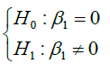
• H0: There is no meaningful relationship between the systemic risk criteria and previous corporate returns.
• H1: There is a significant relationship between the systematic risk measure and the company’s previous returns.
This hypothesis is estimated using model (1) as panel data and will be approved if the coefficient is significant at 95% confidence level.
Ri,t = α0 + β1(Risk Measure)i,t + β2Ln(Size)i,t +β3Ln(B/M)i,t + β4(Tda)i,t + β5Re tNEGi,t + β6(Re tPos * Risk Measure)i,t + εi,t
 (1)
(1)
To determine if the panel data approach is useful in estimating the model, it is necessary to use Chow/F test and to determine which method (fixed effects or random effects) is more suitable for estimation (determining fixed or randomness of the differences between sectional units Hausman test is used. The results of these tests are presented in Table 7. According to the results of Chow test and its P-value (0.0000), the test hypothesis was rejected at the 95% confidence level, indicating that panel data can be used. Also, according to the results of the Hausman test and its P-Value (0.0009) which is less than 0.05, the test hypothesis is rejected at a 95 % confidence level and the hypothesis is accepted. Therefore, it is necessary to estimate the model using the fixed effects method.
| Test | Number | Statistic | Statistic value | Degree of freedom | P-Value |
|---|---|---|---|---|---|
| Chow | 630 | F | 3.0535 | -104.519 | 0 |
| Hausman | 630 | χ2 | 22.7679 | 6 | 0.9 |
Table 7: Chow and Hausman test results for model (1).
In order to measure the validity of the model and to examine the assumptions of the classical regression, it is necessary to study the absence of collinearity between the independent variables entered in the model. In addition, some tests regarding the normality of the residuals, homogeneity of the variances, the independence of the residuals, and the absence of model specification error (linearity of the model) need to be done. To test the normality of error sentences, various tests can be used. One of these tests is the Jarque-Bera test, which is used in this study. The results of the Jarque-Bera test indicate that the residuals from the estimation of the research model have a normal distribution at 95% confidence level, so the probability of this test (0.8214) is greater than 0.05. Another statistical assumption of classical regression is the homogeneity of variance of the residuals. If the variances are not homogeneous, the linear estimator is unbiased and will not have the least variance. In this study, Breusch–Pagan test was used to check the homogeneity of variances. Given the significance level of this test, which is less than 0.05 (0.0000), the null hypothesis stating the existence of the homogeneity of variance is rejected and it can be said that the model has heterogeneity of variance problem. In this study, the generalized least squares estimation (GLS) method has been used to solve this problem. In this study, the Durbin-Watson test (D-W) was used to test the non-correlation of residuals, which is one of the assumptions of regression analysis, and is called self-correlation. According to the preliminary results of the model estimation, the value of Durbin-Watson statistic is 2.07 and since it is between 1.5 and 2.5, it can be concluded that the residuals are independent of each other. In addition, to test whether the model has a linear relationship and whether the research model is properly explained in terms of linearity or non-linearity, Ramsey test has been used. Considering that the significance level of Ramsey test (0.2145) is greater than 0.05, therefore, the null hypothesis of this test assuming the linearity of the model is confirmed and the model has no specification error. The results of the above tests are summarized in Table 8.
| Jarque-Bera Statistic | Breusch-Pagan Statistic | Durbin-Watson Statistic | Ramsey Statistic | |||
|---|---|---|---|---|---|---|
| χ2 | (P-Value) | F | (P-Value) | D | F | (P-Value) |
| 1.9127 | 0.8214 | 29.9661 | 0 | 2.07 | 1.4551 | 0.2145 |
Table 8: Results of the tests regarding the statistical assumptions of model (1).
According to the results of Chow and Hausman tests as well as the results of the test of statistical assumptions of classical regression, model (1) of the research is estimated using the panel data method and as a fixed effect. The estimated model results are presented in Figure 5. The estimated shape of the model using Eviews 7 software will be as follows:
Ri,t = 0.2666+ 0.0781(Risk Measure)i,t -0.2117Ln(Size)i,t + 0.6286(Re tPos * Risk Measure)i,t + εi,t
Results of estimating model 1 by GLS method
Mode1: Ri,t = α0 + β1(Risk Measure)i,t + β2Ln(Size)i,t +β3Ln(B/M)i,t + β4(Tda)i,t + β5Re tNEGi,t + β6(Re tPos * Risk Measure)i,t + εi,t
Mode2: HRi,t = α0 + β1(Risk Measure)i,t + β2Ln(Size)i,t +β3Ln(B/M)i,t + β4(Tda)i,t + β5Re tNEGi,t + β6(Re tPos * Risk Measure)i,t + εi,t
Where, the company i’s previous returns in year t (Ri,t). Expected returns of company i in year t (HRi,t). The systematic risk measure of company i in year t ((Risk Measure)i,t). The size of company i in year t (Ln(Size)i,t). Company i’s growth opportunities in year t (Ln(B/M)i,t). The ratio of stock trades of company i in year t ((Tda)i,t). The negative return of company i in year t (Re tNEGi,t). The contrast between the previous returns and the risk of company i of year t ((Re tPos * Risk Measure)i,t).
In studying the significance of the whole model, considering that the probability of F statistic is smaller than 0.05 (0.000), with the confidence level of 95%, the significance of the whole model is confirmed. The coefficient of determination also indicates that 83.41% of the companies’ previous returns are explained by the variables entered in the model.
In order to study the significance of the coefficients according to the results presented in Table 9, since the probability of t statistic for the coefficient of variable of the systematic risk factor is less than 0.05 (0.0000), the existence of a significant relationship between the systematic risk factor and previous returns at the confidence level of 95% is confirmed. Therefore, the first hypotheses of the research are accepted and it, with 95% confidence, can be said that there is a significant relationship between the systematic risk factor and previous returns. The positive coefficient of this variable (0.0781) indicates a direct relationship between the systematic risk factor and previous returns, in a way that, with the increase of one unit of systematic risk factor the previous returns will increase by 0.0781 units. Therefore, according to the analyses carried out in relation to the confirmation of the first hypothesis of the research, it can be concluded that there is a meaningful and direct relationship between the systematic risk measure and the company’s past performance.
| Dependent Variable: Previous returns Number of observations: 630 year-company | ||||
|---|---|---|---|---|
| Variable | Coefficient | t statistic | P-Value | Relationship |
| Fixed element | 0.2666 | 4.7031 | 0 | Positive |
| Systematic risk factor | 0.0781 | 14.5241 | 0 | Positive |
| Company size | -0.2117 | -2.6913 | 0.0073 | Negative |
| Growth Opportunities | 0.009 | 0.7915 | 0.429 | Insignificant |
| Ratio of stock trades | 0.0007 | 0.0382 | 0.9695 | Insignificant |
| Negative return | 0.0051 | 1.3063 | 0.192 | Insignificant |
| Contrast of previous returns and risk | 0.6286 | 34.5271 | 0 | Positive |
| Coefficient of model determination | 0.8341 | |||
| F Statistic | 23.7284 | |||
| (P-Value) | 0 | |||
Table 9: Results of testing the first hypothesis using fixed effects method.
Results of the test of the second research hypothesis: The purpose of the second hypothesis test is to investigate whether there is a meaningful relationship between the systemic risk criteria and the expected returns of firms. And its statistical hypothesis is as follows:
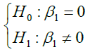
• H0: There is no meaningful relationship between the systemic risk criteria and the expected returns of the companies.
• H1: There is a significant relationship between the systemic risk criteria and the expected returns of the companies.
These hypotheses are estimated using the model (2) as panel data and will be approved if the coefficient is significant at 95% confidence level.
There is a significant relationship between the systemic risk criteria and the expected returns of the companies.
 (2)
(2)
The results of the Chow test (to determine the use of panel or mixed data methods) and Hausman test (to determine the use of the fixed or random effects method in panel data method) for models (2) are presented in Table 10.
| Test | Statistic | Statistic value | Degree of freedom | P-Value |
|---|---|---|---|---|
| Chow | F | 1.644 | -104.519 | 0 |
| Hausman | χ2 | 5.9543 | 6 | 0.9 |
Table 10: Chow and Hausman test results for model (2).
According to the results of Chow test and its P-Value (0.0002), the test hypothesis is rejected at the 95% confidence level, indicating that panel data can be used. Also, according to the results of the Hausman test and its P-Value test (0.0283) which is less than 0.05, the hypothesis is rejected at the 95% confidence level and the hypothesis is accepted. Therefore, it is necessary to estimate the model using the fixed effects method. In examining the classical regression assumptions, the results of the Jarque-Bera test indicate that the residuals of estimating the research model is normally distributed at 95% confidence level in a way that the probability of this test (0.7214) is greater than 0.05. Considering the significance level of the Breusch–Pagan test, which is smaller than 0.05 (0.0114), the null hypothesis stating the existence of variance homogeneity is rejected and it can be said that the model has a variance heterogeneity problem. On this hypothesis, the generalized least squares estimation (GLS) method has been used to eliminate this problem. In the self-correlation test of the residuals of the model carried out by Durbin–Watson test (DW), Durbin–Watson statistic was 2.49. Since it is between 1.5 and 2.5, it can be concluded that the residuals are independent of each other. Moreover, considering that the significance level of Ramsey Test is greater than 0.05, (0.623), therefore, the null hypothesis of this test is stating the linearity of the model is confirmed and the model has no specification error. The summary of the results of the above tests is presented in Table 11.
| Jarque-Bera Statistic | Breusch-Pagan Statistic | Durbin-Watson Statistic | Ramsey Statistic | |||
|---|---|---|---|---|---|---|
| χ2 | (P-Value) | F | (P-Value) | D | F | (P-Value) |
| 1.8599 | 0.7214 | 2.5737 | 0.0114 | 2.49 | 14.7217 | 0.6523 |
Table 11: The results of the tests related to statistical assumptions of the model (2).
According to the results of Chow and Hausman tests as well as the results of the test of statistical assumptions of classical regression, model (2) of the research is estimated using the panel data method as fixed effects. The results of the model estimation are presented in Table 11.
Results of estimation of model 2 by GLS method
Mode1: Ri,t = α0 + β1(Risk Measure)i,t + β2Ln(Size)i,t +β3Ln(B/M)i,t + β4(Tda)i,t + β5Re tNEGi,t + β6(Re tPos * Risk Measure)i,t + εi,t
Mode2: HRi,t = α0 + β1(Risk Measure)i,t + β2Ln(Size)i,t +β3Ln(B/M)i,t + β4(Tda)i,t + β5Re tNEGi,t + β6(Re tPos * Risk Measure)i,t + εi,t
Where, the company i’s previous returns in year t (Ri,t). Expected returns of company i in year t (HRi,t). The systematic risk measure of company i in year t ((Risk Measure)i,t). The size of company i in year t (Ln(Size)i,t). Company i’s growth opportunities in year t (Ln(B/M)i,t). The ratio of stock trades of company i in year t ((Tda)i,t). The negative return of company i in year t (Re tNEGi,t). The contrast between the previous returns and the risk of company i of year t ((Re tPos * Risk Measure)i,t).
The estimated shape of the model will be as follow:
HRi,t = 0.5827+ 0.0946(Risk Measure)i,t +0.2907(Tda)i,t + 0.8773(Re tPos * Risk Measure)i,t + εi,t
In studying the significance of the whole model, given that the probability of the F statistic is smaller than 0.05 (0.0000), with a confidence level of 95%, the whole model’s significance is confirmed. The model’s determination coefficient also indicates that 44.30% of the expected return is defined by the variables entered in the model.
According to the results presented in Table 12, since the probability of the t statistic for the coefficient of variance of the systematic risk factor is less than 0.05 (0.0000), the existence of a significant relationship between the systemic risk factor and the expected returns is verified at 95% confidence level. Therefore, the second research hypothesis is accepted and, with 95% confidence, it can be said that there is a significant relationship between the systematic risk factor and the expected return. The coefficient of this variable being positive (0.946), there is a direct relationship between the systematic risk factor and the expected return, such that with an increase of 1 unit in the systematic risk factor, the expected return will increase by 0.946 units. Therefore, according to the analysis done regarding the confirmation of the second research hypothesis, it can be concluded that there is a significant and direct relationship between the systematic risk factor and the expected return of the companies.
| Dependent Variable: Previous returns Number of observations: 630 year-company | ||||
|---|---|---|---|---|
| Variable | Coefficient | t statistic | P-Value | Relationship |
| Fixed element | 0.5827 | 2.5351 | 0.0115 | Positive |
| Systematic risk factor | 0.0946 | 3.6363 | 0.0003 | Positive |
| Company size | -0.1836 | -0.5688 | 0.5697 | Negative |
| Growth Opportunities | -0.1093 | -1.8657 | 0.0626 | Insignificant |
| Ratio of stock trades | 0.2907 | 2.3139 | 0.0211 | Insignificant |
| Negative return | -0.0224 | -1.1387 | 0.2553 | Insignificant |
| Contrast of previous returns and risk | 0.8773 | 11.5418 | 0 | Positive |
| Coefficient of model determination | 0.443 | |||
| F Statistic | 3.7529 | |||
| (P-Value) | 0 | |||
Table 12: Results of the test of the second research hypothesis using fixed effects method.
Considering that in both models, there is a positive and significant relationship between the systemic risk criteria and the initial yields and expected returns of the companies. It can be said that there is a direct and significant relationship between the expected returns and the expected returns. Based on the Pearson correlation coefficient (Table 6), it can be said that there is a positive correlation between the two variables at the confidence level of 99%. In the event of an increase in the previous yields, the expected returns will also increase. But, in comparison with the coefficient determined in the two regression estimation models, the first model with a deterioration of 83% has more explanatory power than the systematic risk criterion as the predictor of previous outcomes in relation to expected returns.
The results of the hypotheses
Test results of the first hypothesis of the research: Considering that the probability of F statistics is smaller than 0.05 (0.0000), with the confidence of 95%, the significance of the whole model is confirmed. The coefficient of model determination also indicates that 83.41% of the company’s previous returns are explained by the variables entered in the model. With respect to the results presented in Figure 5, the probability of the t statistic for the coefficient of variance of the systematic risk factor is less than 0.05 (0.0000), so the existence of a significant relationship between the systemic risk factor and previous returns at 95% confidence level is confirmed. Therefore, the first hypotheses of the research are accepted and, with 95% confidence, it can be said that there is a significant relationship between the systematic risk factor and previous returns. The positivity of the coefficient of this variable (0.0781) indicates a direct relationship between the systemic risk factor and previous returns, such that with an increase of one unit in systematic risk factor, the previous returns will increase by 0.0781 units. Therefore, according to the analyzes carried out in relation to the confirmation of the first hypothesis of the research, it can be concluded that there is a significant and direct relationship between the systemic risk criteria and the previous company’s returns.
The result of the first hypothesis stating a significant relationship between the independent and dependent variables accords with the research of Bali et al. [7] and Beckert et al. [8], but in terms of the type of relationship (direct or inverse) agrees with the results of the Tsai et al. [9] research, but contradicted by Gregory et al. [10].
Test results of the second hypothesis of the research: Considering that the probability of F statistics is smaller than 0.05 (0.0000), with the confidence of 95%, the significance of the whole model is confirmed. The coefficient of model determination also indicates that 44.30% of the companies’ previous returns are explained by the variables entered in the model. With respect to the results presented in Figures 5-7, the probability of the t statistic for the coefficient of variance of the systematic risk factor is less than 0.05 (0.0000), so the existence of a significant relationship between the systemic risk factor and the expected returns is confirmed at 95% confidence level. Therefore, the second hypotheses of the research are accepted and, with 95% confidence, it can be said that there is a significant relationship between the systematic risk factor and expected returns of the companies. The positivity of the coefficient of this variable (0.0946) indicates a direct relationship between the systemic risk factor and the expected returns, such that with an increase of one unit in systematic risk factor, the expected returns will increase by 0.0946 units. Therefore, according to the analysis done in conjunction with the confirmation of the second hypothesis of the research, it can be concluded that there is a meaningful and direct relationship between the systematic risk criteria and expected returns of the companies.

Figure 6: Results of estimating model 1 by GLS method.

Figure 7: Results of estimation of model 2 by GLS method.
The results of our second hypothesis are consistent with the findings.
Research Constraints
The basis of each research is the information that the research hypotheses are tested using. Obviously, the more accurate and complete the information is available to the researcher, the results of the research are also more reliable and the research carried out will be more credible.
1. One of the research limitations is the discrepancy between the statistical information reported by the website of the Stock Exchange Company and the information contained in data banks. In the present case the information provided by the Stock Exchange Company and its website was relied on.
2. The information gathered in this research included the companies accepted in Tehran Stock Exchange between 2010 and 201. As with the increase of information and the number of observations the test results and thus the result of the research will have a higher validity, different results may be obtained with the increase of the study period.
3. Although the data was collected through much effort and care, because of poor data sources, a few companies were excluded from the test samples, especially on previous returns and the expected return of the companies.
Proposals based on research results
1. According to the results of this research and similar investigations, the Stock Exchange Company can publish more comprehensive information about the previous returns and expected returns for shareholders.
2. Recommending those references in charge of drafting accounting standards to voluntarily disclose comprehensive information on the level of systematic risk factor and previous and expected returns of firms.
3. Because the increase in the level of systematic risk factor can have significant effects on the decision of investors, providing complete and transparent information by management about systematic risk factor, previous returns and expected returns will be highly groundbreaking.
4. It would be better if financial analysts active in the capital market and investment advisors in the stock market utilized, along with the usual analyses and techniques, specific analyses based on the status of previous and expected returns and the factors affecting them, and also the systematic risk factor of companies considering accounting standards.
5. Studying the impact of industry type on the impact of systematic risk factor, previous returns and expected returns of firms.
6. Using other control variables such as industry index and credit rating, in examining the impact of systematic risk factor on previous returns and expected returns of companies.
7. Investigating the impact of macroeconomic variables such as: inflation, oil price and the currency rate on the identification of the effect of systematic risk factor on previous returns and expected returns of companies.
References
- Mukharji D, Harun-Ar-Rashid M, Pattanaik SS, Datta S (2011) INDIA AND BANGLADESH-A NEW PHASE IN BILATERAL RELATIONS. Indian Foreign Aff J 6: 365.
- Atmadja AS (2005) The Granger Causality Tests For The Five ASEAN Countries Stock Markets And Macroeconomic Variables During And Post The 1997 Asian Financial Crisis. Jurnal Manajemen dan Kewirausahaan 7: 1.
- Blitz D, Van Vliet P (2007) The volatility effect: Lower risk without lower return. J Portfolio Manag 1: 102-113.
- Brown RL, Durbin J, Evans JM (1975) Techniques for testing the constancy of regression relationships over time. J R Stat Soc 1: 149-192.
- Baker M, Bradley B, Wurgler J (2011) Benchmarks as limits to arbitrage: Understanding the low-volatility anomaly. Financ Anal J 67: 40-54.
- Goyal A, Santaâ€ÂÂÂClara P (2003) Idiosyncratic risk matters!. The J Fin 58: 975-1007.
- Bali TG, Peng L, Shen Y, Tang Y (2013) Liquidity shocks and stock market reactions. The Review of Financial Studies 27: 1434-1485.
- Beckert J (2009) The social order of markets. Theory and society 38: 245-269.
- Namazi M, Kermani E (2013) An empirical investigation of the relationship between corporate ownership structures and their performances (Evidence from Tehran Stock Exchange). Journal of Finance and accounting 1: 13-26.
- Chow GC (2006) Globalization and China's economic development. Pacific Economic Review 11: 271-285.