Spanish
  Chinese
  Russian
  German
  French
  Japanese
  Portuguese
  Hindi
Hindi Research Article, J Appl Bioinformat Computat Biol S Vol: 10 Issue: 3
A Mathematical Model for the Dynamics of Rhinopharyngitis in a Population
Ernest Danso-Addo* and Joseph Acquah
Department of Mathematical Sciences, Faculty of Engineering, University of Mines and Technology, Tarkwa, Ghana
*Corresponding Author: Ernest Danso-Addo
Department of Mathematical Sciences, Faculty of Engineering, University of Mines and Technology, Tarkwa, Ghana
E-mail: edanso-addo@umat.edu.gh
Received: September 28, 2021 Accepted: October 18, 2021 Published: October 25, 2021
Citation: Danso-Addo E, Acquah J (2021) A Mathematical Model for the Dynamics of Rhinopharyngitis in a Population. J Appl Bioinforma Comput Biol S4.
Abstract
This paper considered a deterministic SIR model to investigate the transmission dynamics of common cold within a population. This study was based on the assumption that every individual in the population is susceptible to the common cold. The steady states of the model were calculated and the local and global asymptotic stability analyzed. The basic reproduction number R0 was determined. The disease becomes endemic whenever R0>1 and dies out whenever R0<1. Simulations of the model were performed. It was found that the transmission rate is most sensitive to the disease; any attempt to reduce the transmission rate is marked by a reduction in the number of infectious individuals.
Keywords: Basic Reproduction Number; Steady States; Local and Global Stability; Common Cold; Simulation; Rhinopharyngitis
Introduction
The common cold or upper respiratory tract infection is a mild viral infectious disease caused by more than 200 virus strains. Since so many different viruses can cause common cold infection and new common cold virus strains do constantly develop, the body never accumulates enough resistance against them [1,2]. For this reason, colds are a frequent and recurring problem. Common cold infection is the most recurrent human disease and affects people all over the globe [3]. It is the leading cause of doctor visits and missed days from school and work. Each year, children can have between 6–12 colds whereas adolescents and adults typically have between 2-3 colds [1]. The National Institute of Allergy and Infectious Diseases (NIAID) in 2012 estimated that individuals in the United States suffer about 100 million colds annually with approximately 22 million days of school absences and 150 million workdays lost in the United States alone [4].
No vaccine or cure for cold exists but measures exist that can help relieve the body of its symptoms [5]. However, this infection if unattended can linger and break down the body’s defenses and lead to bronchitis, ear infection, sinusitis, and other serious complications such as pneumonia in people with weakened immune systems. According to the World Health Organization (WHO), respiratory tract infections are among the most important human health problems because of their high incidence and consequent economic cost. In the United States, the common cold leads to 75-100 million Physician visits annually at a conservative cost estimate of $7.7 billion per year [3]. Drug therapy for common colds produces few measurable benefits and antibiotic treatment does not shorten the duration of the illness or prevent the development into pneumonia. This has therefore necessitated the need to develop a mathematical model for the common cold and study its dynamics.
Common cold or simply cold referred to as acute viral rhinopharyngitis or acute coryza is a viral infectious disease of the upper respiratory tract, which primarily affects the nose, the throat, and the sinuses. Although cold is usually mild, it can break the body’s defenses and present uncomfortable symptoms such as coughing, sore throat, runny nose, sneezing, fever, watery eyes, and congestion. Since anyone or well over 200 viruses can cause a cold, signs and symptoms tend to vary greatly. The most familiar categories of cold viruses include rhinoviruses, coronaviruses, and adenoviruses [5,6]. Moreover, symptoms that occur are mostly due to the body’s immune response to the infection rather than to tissue destruction by the viruses themselves. No cure or vaccine exists to help fight against Upper Tract Respiratory Infection (UTRI), but it can be prevented significantly by frequent hand washing. In addition, the symptoms can be treated, however, these infections, if not properly managed can lead to bronchitis, sinusitis, ear, and even pneumonia in people with weakened immune systems [6].
UTRI is the most frequent infectious disease in humans with the average adult getting between 2-3 colds per year and the average child having between 6-12 colds [7]. The common cold is a self-limited condition and is generally managed at home [1].
The symptoms of the common cold usually appear about one to three days after exposure to a cold-causing virus [4]. Typical symptoms include cough, runny or stuffy nose, sore throat, nasal congestion, slight body aches, mild headache, and fatigue. Others are watery eyes, loss of appetite, low-grade fever, and sneezing. A sore throat may be present in about 40% of the cases whereas a cough and a muscle ache may occur in about 50% of the cases. Generally, a fever may not be present in adults but it is very common in infants and young children. The discharge from the nose may become thicker and yellow or green as the common cold progresses. This does not indicate the virus strain causing the cold.
There are measures in place to help relieve the body of common cold symptoms. However, if these symptoms are not properly managed, they can linger and break down the body’s defenses and lead to the following Acute Ear Infection (Otitis media): ear infection occurs when bacteria or viruses infiltrate the space behind the eardrum [4].
A cold often begins with a tickle in the throat, a feeling of being chilled, sneezing, and headache, followed by a runny nose and cough in a couple of days. Symptoms may begin within 16 hours of exposure and typically peak two to four days after onset. Colds usually resolve in seven to ten days but some can prolong, lasting about two to three weeks.
The rhinovirus is the most responsible cause of UTRI and is known to cause 30 – 80% of all colds globally. It is highly contagious and is responsible for making people sneeze and sniffle [4]. Other commonly implicated viruses include human coronavirus (causes approximately 15% of colds), influenza virus (causes10-15% of colds), adenovirus (causes 5% of colds), human parainfluenza virus, human respiratory syncytial virus, and metapneumovirus.
A cold virus enters the body through the mouth, eyes, or nose [4]. The virus is transmitted via airborne droplets when someone with the common cold coughs, talks, or sneezes. It can also spread from person to person by coming into direct contact with contaminated objects such as utensils, stationery, towels, computers, toys, telephones, and doorknobs [8]. The virus may survive for prolonged periods in the environment (over 18 hours for rhinoviruses) and can be picked up by people’s hands and subsequently carried to their eyes or nose where infection occurs [4].
Nickbaksh [9] considered co-circulatory viruses that are accountable for acute respiratory infections. They analyzed diagnostic data from 44230 cases of respiratory illnesses. Key to their analysis was accounting for alternative drivers of correlated infection frequency. In mathematical simulations that mimic 2- pathogen dynamics, they showed that transient immune-mediated interference can cause coldlike viruses to diminish during peak activity of a seasonal virus.
Model Formulation
In this paper, a deterministic mathematical model is formulated to describe the transmission of the common cold in a human population. This population is further compartmentalized into epidemiological classes as shown below Figure 1.

Figure 1: Compartmentalized model of the common cold.
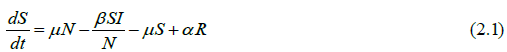
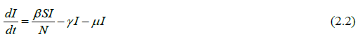
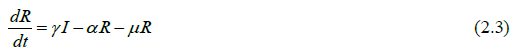
The susceptible population is designated as S(t) The number of the infected population is denoted by whiles the recovered individuals are represented by R(t). The recruitment rate of the population is μ and the total number of new births is denoted by μN. The contact rate β is the rate at which susceptible individuals come into contact with the infected population. The recovery rate is the rate of progression from the infectious class to the recovery class. The per capita loss of immunity is given by α
Assumptions of the Model
i) Every individual in the population is susceptible to common cold infection.
ii) There are no deaths as a result of catching a cold.
iii) There is no progression from the susceptible class into the exposed class because one becomes infectious after catching a cold virus.
iv) The natural death rate is equivalent to the birth rate because of the short duration of the disease.
v) Recovered individuals have temporarily induced immunity
Formulated Model Equation
The following systems of differential equations are formulated from the compartmental model diagram above to mimic the dynamics of the common cold.
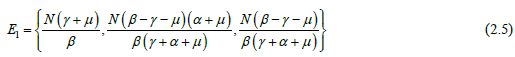
Equilibrium Solutions
The steady states of the system of differential equations in Equations (2.1) to (2.3) is attained by equating the system off to zero and solving to get the disease-free, E0 and the endemic equilibrium E1 in Equations (2.4) and (2.5) as follows:

Determination of the Basic Reproduction Number (R0)
For the computation of R0, it is crucial to distinguish new infections from all other changes in the population. From Equation (2.2) the disease state at equilibrium is given by Equation (2.6).
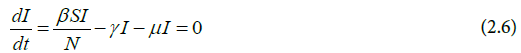
At the onset of the disease, nearly everyone is susceptible to infection. Thus, the number of susceptible individuals is equal to the total population; S=N. Substituting this into (2.6) gives;
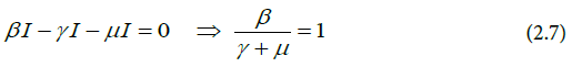
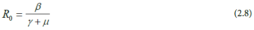
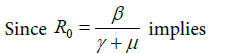
Hence, the basic reproduction number is calculated as
Local Asymptotic Stability of the Disease Free Equilibrium
The stability analysis for the system of Equations (2.1) to (2.3) is outlined in this section. The disease-free equilibrium in Equation (2.4) is locally asymptotically stable if and only if R0 >1 [8].
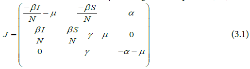
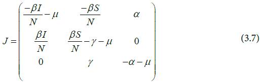
The Jacobian matrix of the system is given in Equation (3.1).
The Jacobian J, evaluated at the disease-free equilibrium, E0 is represented in the array below.
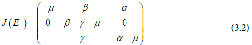
The characteristic polynomial of the Jacobian matrix in Equation (3.2) is given in Equation (3.3).

The solution to the characteristic polynomial (3.3) gives the following eigenvalues;


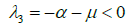
The disease-free equilibrium is locally asymptotically stable provided all eigenvalues are negative. Items λ1 and λ3 are negative. Hence imposing a negativity condition on λ1 2 gives:

This implies that  . Dividing through by the right hand
side gives Equation (3.5)t
. Dividing through by the right hand
side gives Equation (3.5)t
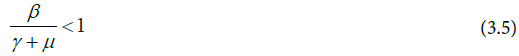

Therefore, the disease-free equilibrium is proven to be locally asymptotically stable provided R0< 1
Local Asymptotic Stability of the Endemic Equilibrium
The endemic equilibrium in Equation (2.5) is locally asymptotically stable if and only if R0>1 [8].
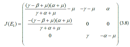
The Jacobian matrix of the system is given by
The Jacobian J, evaluated at the endemic equilibrium E1 is represented in the array below
Equation (3.9) is the characteristic polynomial of Equation (3.8).
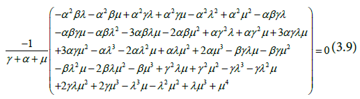
The solution to the characteristic polynomial (3.9) gives the following eigenvalues;


and
From Equations (3.10) and (3.12), it is clearly evident that 
 to be negative,


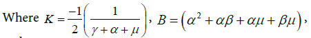
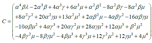
Substituting for the expressions of B and C and factorising yields Equation (3.16).


Therefore, the Endemic Equilibrium is locally asymptotically stable provided R0 >1.
Global Asymptotic Stability
The global asymptotic stability was carried out for the disease-free equilibrium and the endemic equilibrium.
Global Asymptotic Stability of the Disease-Free Equilibrium
The global asymptotic stability of the disease-free equilibrium was proven by the theorem below.
Theorem 4.1
If R0 ≤1, then the disease-free equilibrium is globally asymptotically stable in the Domain.
Proof
 by the Lyapunov function

Differentiating the Lyapunov function gives

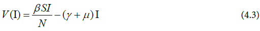
From Equation (2.2), we obtain Equation (4.3).
Equivalently,

Further simplification yields 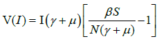
At the disease-free equilibrium, the susceptible population, S = N , the total population. Hence,

Therefore, V (I ) ≤ 0 provided R0 ≤1.
Hence, the disease-free equilibrium is globally asymptotically stable.
Global Asymptotic Stability of the Endemic Equilibrium
In this subsection, the global stability of the Endemic Equilibrium is proven by the use of the Lyapunov function.
Theorem 4.2
The endemic equilibrium in equation 4.3 is globally asymptotically stable in the domain ϕ if and only if R0 >1.
Proof
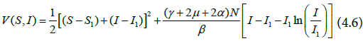
Let consider the Lyapunov function candidate of the form 
Then, V is C1 on the interior of ϕ , E1 is the global minimum of  Differentiating the Lyapunov function
V gives
Differentiating the Lyapunov function
V gives
Simplifying further,
Hence,
At the equilibrium,  which implies
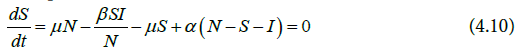
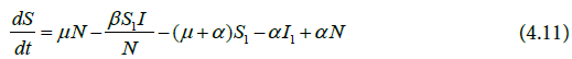
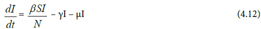
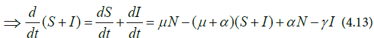
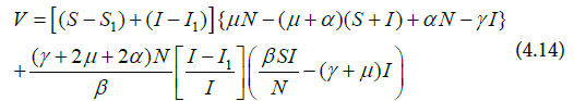
Substituting Equations (4.11) to (4.13) into Equation (4.9) gives Equation (4.14)
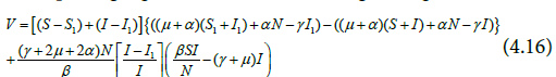
At the steady states,

Thus, putting Equation (4.15) into (4.14) gives Equations (4.16).
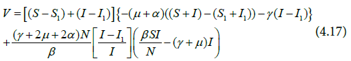
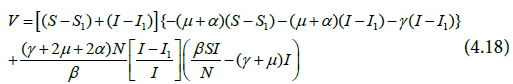
Further simplification of Equation (4.16) yields Equation (4.17) and (4.18).
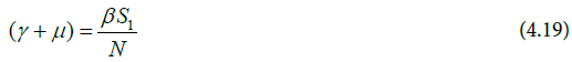
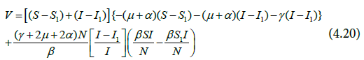
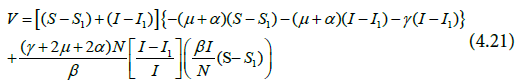
Again, making the assumption in Equation (4.19) and substituting it into Equation (4.18) we have the following:
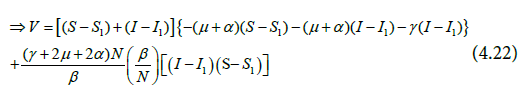
Expanding and simplifying the Equation (4,23) gives Equation (4.24).
Rearranging and simplifying yields Equation (4.25) and (4.26).
Hence V ≤ 0.V=0 If and only if S = S* and I = I* . Therefore, the Endemic Equilibrium is globally asymptotically stable in the interior of ϕ .
Simulation and Analysis of the Common Cold Model
Numerical simulations are carried out to give graphical representations of the model. Estimated parameter values are shown in Table 1. The parameter values were estimated using different sources of literature [10-12].
| Parameter | Parameter value |
|---|---|
| µ | 0.0000456 per day (Estimated) |
| β | 0.5per day (Estimated) |
| γ | 0.01176470588 per day (Estimated) |
| α | 0.01095890411 per day (Estimated) |
Table 1: Parameter Values for the Model.
Numerical Simulation of the Model
The following graphs are the solution curves of the system of differential equations (4.1) to (4.3).
Discussion the Model
Figure 2 shows the interaction of the evolution of the common cold infection in an entire population. An introduction of infectives into the population leads to a rapid decline in the number of susceptible individuals. This is as a result of a higher effective contact rate As the disease goes through the population, the susceptible population declines and attains a minimum. As the susceptible class decreases, the number of infected individuals increases initially due to the spread of the common cold and becomes endemic. Figure 3 shows the numerical simulation of the susceptible individuals. The common cold infection is a self-limited disease (Infectious individuals recover in a short while) and recovery from the disease does not confer permanent immunity. The number of susceptible individuals begins to rise again and fluctuates as some of the recovered individuals catch the disease again. This phenomenon continues until it reaches a threshold where the disease becomes endemic in the population.

Figure 2: The solution curves showing the evolution of the disease and the interaction among the state variables.

Figure 3: Evolution of the susceptible individuals.
In Figure 4, the absence of the disease at the initial stage is the reason why the infectious class is zero. Once an epidemic starts, the infectious class grows exponentially as more individuals from the susceptible class join the infectious class due to a higher effective contact rate. The number of infectious individuals then decreases sharply because of the shorter life span of the common cold. This results in an increase in the number of susceptible individuals. The infectious population increases up to the peak of the disease and decreases becomes asymptotic to the horizontal.

Figure 4: Evolution of the infected population.
Figure 5 is a direct consequence of Figure 4. It represents the numerical simulation of the Recovered class at given times. When common cold is introduced into the susceptible population the number of recovered individuals rises exponentially with time since the common cold infection has a shorter life span and more individuals recover from the disease. Almost the total population recovers from common cold infection eventually. Recovery from common cold disease does not confer permanent immunity.

Figure 5: Simulation of the Recovered Individuals.
The Simulation of the model to determine the sensitivity of the transmission rate is shown in Figure 6. Various parameters were examined against the disease (Common Cold) to check which parameter is more sensitive. The results showed that the transmission rate is the most sensitive, with the other parameters being slightly sensitive. It can be seen from (Figure 5) that any attempt to reduce the transmission rate is marked by a reduction in the number of infectious individuals. At transmission rate β=0.1 ( ), it is observed that the disease eventually dies out in the long run. At contact rate β=0.3 through to 0.8 in which case >1, it is observed that the infection can spread in the population.

Figure 6: Simulation to Show the Sensitivity of the Transmission Rate on the Disease.
Conclusion
In this paper, a deterministic mathematical model for rhinopharyngitis has been formulated and its dynamics duly investigated. From the model, the basic reproduction number was derived. The disease-free equilibrium, E0, was calculated and found to be locally asymptotically stable whenever R0<1. The endemic equilibrium E1 was also found to be locally asymptotically stable whenever R0>1. Lyapunov functions were used to establish that the steady states are globally asymptotically stable.
The model was simulated to ascertain the evolution of the disease and performed sensitivity analysis on the basic reproduction number from which it was concluded that the parameter β is the most sensitive.
Due to the relative mildness of the common cold infection, proper attention has eluded it, yet the economic impact is enormous. Proper personal hygiene if practiced will effectively retire the disease.
References
- Doerr S, Gompf SG (2020) Common Cold: Symptoms, Treatment, Causes, vs Flu, Duration and Prevention. Available from https://www.medicinenet.com/common_cold/article.html.
- https://www.medicinenet.com/common_cold/article.html.
- Goldman R, Watson S (2020) The Difference between Cold and flu. Retrived from http://www.healthline.com/health/cold-flu/cold-or-flu.
- Mayo Clinic (2020) Diseases and Conditions: Common cold. Available from https://www.mayoclinic.org/diseases-conditions/common-cold/symptoms-causes/syc-20351605.
- Pappas DE (2018) Principles and Practice of Pediatric Infectious Diseases: The Common Cold. Elsevier 199 – 202.
- Boncristiani HF, Criado MF, Arruda E (2009) Respiratory Viruses. Encyclopedia of Microbiology 500–518. https://doi.org/10.1016/B978-012373944-5.00314-X
- Michael P (2017) All bout Common the Cold. Available from https://www.medicalnewstoday.com/articles/166606.
- http://www.healthline.com/health/cold-flu/cold-or-flu.
- https://www.mayoclinic.org/diseases-conditions/common-cold/symptoms-causes/syc-20351605.
- Lumen Microbiology (2020) Viral infections of the respiratory tract. Available from https://courses.lumenlearning.com/microbiology/chapter/viral-infections-of-the-respiratory-tract/.
- CDC (2019) Common cold: protect yourself and Others. Available From https://www.cdc.gov/features/rhinoviruses/index.html.
- Allen JS (2007) An Introduction to Mathematical Biology. Pearson Education Inc., New Jersey, USA 174- 176.