Spanish
  Chinese
  Russian
  German
  French
  Japanese
  Portuguese
  Hindi
Hindi Research Article, Jceit Vol: 10 Issue: 5
A Study on Spectrum Based Fault Localization Techniques
Saksham Sahai Srivastava*
Department of Chemical Engineering, Indian Institute of Technology Kharagpur, India
Corresponding Author:
Saksham Sahai Srivastava
Department of Chemical Engineering
Indian Institute of Technology Kharagpur, India
E-mail: sakshamsahai4796@iitkgp.ac.in
Received: March 24, 2021 Accepted: April 08, 2021 Published: April 15, 2021
Citation: Srivastava SS (2021) A Study on Spectrum Based Fault Localization Techniques. J Comput Eng Inf Technol 10:4.
Abstract
Fault Localization or debugging is one of the major aspects when it comes to testing activity. In this criterion a fault is located and removed when a failure occurs during test. Many types of techniques were proposed before Spectrum-based Fault Localization (SFL) techniques was proposed in order to address the problem of fault localization, which point out program elements which have susceptibility of containing faults. In this article we will apply three different techniques to the different SBFL formulas. The two techniques are uniqueness and slicing. The third one is the combination of these two techniques. We will compare the efficiency and effectiveness of each of the technique on different Spectrum based Fault Localization techniques which will be applied on seven siemens suite programs
Keywords: Fault localization; Slicing, unique.
Keywords
Fault localization; Slicing, unique.
Introduction
According to Araki [1,2], one of the earliest debugging practices constitutes of developing the code with print statements inserted in between to find out the state of variables. With the advent of advancement, there have been little changes in fault localization in practice over time. The techniques proposed in the 1960s [3-5] and used in today’s world by developers, and earlier debugging tools originate from the late 1950s [4]. The idea of this tool was based on moving the debugging program to the computer’s memory, which helps in verification and modification during the execution. A tool called EXtendable Debugging and Monitoring System (EXDAMS) [6,7] was presented by Balzer, which was capable of navigating both backward or forward navigation through the code. The visualization technique of this tool uses graphics to provide control-flow and dataflow information, which can be like tree structure of execution at some point of interest.
Software fault localization is found to be one of the most time consuming, tedious and expensive activity in debugging of different programs. Leading to a great demand for automatic fault localization techniques that can help and suggest ways to programmers to locate faults, with minimum amount of human intervention. So, there is development of different methods, which makes the fault localization process more effective as well as efficient. The complexity of software and its scale has rapidly increased due to this ongoing trend. So, this increase in complexity of software has led to increase in software bugs which have resulted in huge losses [8-10].
The different techniques used to automate fault localisation are i) Spectrum Based Techniques ii) Machine Learning Techniques iii) Slicing Techniques
Weiser [11,12] proposed the Program Slicing technique. On applying this technique, the fault in the program is confined only in a small region, which is, a relevant slice. Program slicing technique are of two type- static and dynamic. In a program the flow of control and data are analysed statically by means of static program slicing [13,14] (statically) which helps in reduction of search space for locating fault. But due to high conservative nature of static slicing technique, the precision of locating fault is very small. In static program slicing technique, dynamic technique [15,16] the search domain of faults is reduced and therefore we get more precise slicing criterion. The statements in which the value of a variable is influenced for a particular program input are generally considered in a dynamic program slice [15,16]. There are some drawbacks of slicing also, which include- i) Static Slicing considers all possible executions. ii) The current test case that reveals the fault is not taken into account. Although, it is used for gaining debugging information. iii) Static slices comprise too many statements (for a certain test case) iv) Dynamic slicing may not contain the faulty statement.
Behavioural patterns which are associated with the different faults, are identified by the machine techniques. Some of the faults like variable not initialized in programs can be easily identified using machine learning techniques. Some of the machine learning techniques are SVM (Support Vector Machine), Neural Network Based Techniques, BPNN [17-19] (Back Propagation Neural Network), RBFNN [18] (Radial Based Function Neural Networks), DNN [17] (Deep Neural Networks). Support vector machines are one of the supervised learning models of machine learning. In this learning algorithms classification and regression analysis are used to analyse data.
Machine learning literature include neural networks as a class of model. The development of neural networks was a kind of revolution in the field of machine learning. Their specific algorithms are inspired from the biological neural networks and are found to be quite efficient and effective in solving most of the machine learning problems. Neural Networks are dealt with those Machine Learning problem where the problem is about learning a complex mapping from the input to the output space because they are basically complex function approximations. Hence the fault localization techniques are greatly modified to give better results by using neural networks.
A BP neural network [20-21] is basically a feed forward neural network. This network has neurons organized in layers, and each neuron in this layer are connected to the neurons in the next layer. This means that directed cycles do not exist in such a network. A complicated nonlinear input-output function generated from a set of sample data which includes inputs and the corresponding expected outputs is used to train a Back Propagation neural network. The data flow in a BP neural network [21] is delivered from the input layer, through hidden layer(s), to the output layer, without any feedback. This algorithm is an iterative algorithm which adjusts the weights of the network in such a manner that it completely fits the training data. But overtraining the algorithm with a particular set of data may result in over-fitting.
When there are more than one layer of hidden units between the inputs and outputs of the artificial neural network which is feed forward then it is known as deep neural network or DNN [17]. The hidden unit uses the logistic function (the closely related hyperbolic tangent is also often used and any function with a well-behaved derivative can be used) to map its total input from the layer below. DNNs can be discriminatively trained (DT) by backpropagating derivatives of a cost function that measures the discrepancy between the target outputs and the actual outputs produced for each training case [20]. Moreover, they have also largely contributed to present studies and research on fault localization and have proposed methods of locating faults with minimal cost.
Although machine learning techniques also have some disadvantages. There can also be times where they must wait for new data to be generated. This means that additional computer power requirement is there. Interpreting the results generated by the algorithms accurately is another major challenge. The algorithms to perform the operation should also be chosen wisely. It also needs massive resources to function. If we train the algorithm with small data set then we may end up with biased predictions coming from a biased training set. This leads to irrelevant advertisements being displayed to customers.
Many strategies were proposed in spectrum-based fault localization in order to locate buggy portion of the code. These techniques use ranking metrics or statistical techniques to generate suspiciousness score of each of the program entity. Tarantula [21- 23] was one of the first techniques proposed for SFL. Program dependencies, execution graphs, and clustering of program entities are sometimes used by many SFL techniques. Tarantula calculates the frequency in which a program entity is executed in all failing test cases, divided by the frequency in which this program entity is executed in all failing and passing test cases. The results were further improved and DStar [11] formula was developed which is the present state of art. Souza [23-27] showed a survey which discusses the stateof- the-art of SFL, including the different techniques that have been proposed, the type and number of faults they address, the types of spectra they use, the programs they utilize in their validation, the testing data that support them, and their use at industrial settings. But there are some drawbacks of SFL techniques as well, the ranking position may sometimes not be determined exactly, as it can happen that multiple ranked elements share the exact same suspiciousness. In such a situation all elements with the same suspiciousness are randomly ordered. Thus, we will have a best case and a worst case in the final ranking when multiple program elements have same suspiciousness score. In the best case, the faulty element is the first element of all elements with the same suspiciousness to be checked for bug. In the worst case, the faulty element is the last element of all elements with the same suspiciousness to be checked for bug. Whereas the greatest advantage of SFL technique is that they are both effective as well efficient.
This article is divided into various sections.
The section about basic concepts and the preliminaries also include the formulae and general information of the different SBFL techniques used in the article.
The methodology developed by us in order to modify the technique and generate better results are further explained in a Section, also contains the results generated.
Then next Sections consist of the related work and conclusion of this article.
Basic Concepts and Preliminaries
Spectrum based fault localization technique originated with the basic formula of Tarantula [21] which is basically derived from the most basic theorem of probability which is Baye’s theorem. It basically the pass/fail information about each test case, and also information of execution of different source code program segments which include statements, branches and methods for each and every test case. The main intuition behind Tarantula [21] is that entities in a program like statements, branches and methods that are executed by failed test cases are more expected to be faulty than those that are executed by passed test cases. On further research we come across a conclusion that this tolerance often provides for more effective fault localization.
Modification of the Kulczynski coefficient proposed a very effective and efficient fault localization technique called as D * which is the present state of art. Effectiveness of D* is evaluated across 21 programs and compared to 16 different fault localization techniques. Testing the technique of DStar [11] with various test cases it was found out that D * generates better suspiciousness score of different statements in a program and is thus more effective technique than the other methods. Moreover different values of * have different impact on the effectiveness of D* method. Different values in the range of 2 to 50 with a difference of 0.5 (* = 2.0, 2.5, 3.0, ..., 50.0) were examined to locate bugs and it was observed that the total number of statements examined to locate all the bugs in the siemens suite programs declines as the value of the * increases from 2 to 33, and after that the number remains almost the same. Hence the method DStar [11] is the present state of art.
| Ranking Metric | Formula |
|---|---|
| Tarantula | 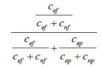 |
| Jaccard | 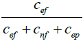 |
| Kulczynski2 | 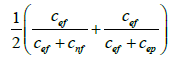 |
| McCon | 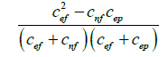 |
| Minus | 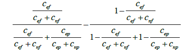 |
| Ochiai | 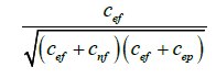 |
| DStar | 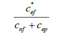 |
| Zoltar | 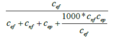 |
Proposed Methodology
In this article, initially we will apply unique technique on different faulty versions. On applying the uniqueness technique, we will get rid of redundant test cases. Hence, the cardinality of test cases reduces and thereafter the technique is improved. The algorithm for the unique technique is as follows in Algorithm 1

Algorithm 1: The algorithm for the unique technique.
Here the matrix ‘Matrix 1’ contains the information of pass/fail of all the test cases and also the information of which all statements are invoked or not invoked for each and every test case. The matrix ‘Matrix 2’ is generated such that it contains only the unique test cases. The rows of the matrix represent different test cases and the columns represent different statements of the program. Let us assume the ‘Matrix 1’ be as follows:
| No | 1 | 2 | 3 | 4 | 5 | 6 | 7 | 8 | 9 | 10 | 11 | 12 | 13 | 14 | 15 | 16 | 17 | 18 | 19 | 20 | R |
| 1 | 1 | 1 | 1 | 1 | 1 | 0 | 1 | 0 | 0 | 1 | 1 | 1 | 0 | 0 | 1 | 0 | 1 | 0 | 1 | 1 | 0 |
| 2 | 1 | 1 | 1 | 0 | 0 | 1 | 0 | 1 | 1 | 0 | 1 | 0 | 1 | 1 | 1 | 1 | 0 | 0 | 1 | 0 | 1 |
| 3 | 1 | 1 | 1 | 1 | 0 | 1 | 1 | 0 | 1 | 1 | 1 | 0 | 0 | 1 | 0 | 1 | 0 | 1 | 1 | 1 | 1 |
| 4 | 1 | 1 | 1 | 1 | 1 | 0 | 1 | 0 | 0 | 1 | 1 | 1 | 0 | 0 | 1 | 0 | 1 | 0 | 1 | 1 | 0 |
| 5 | 1 | 1 | 1 | 0 | 1 | 1 | 0 | 1 | 1 | 1 | 0 | 0 | 1 | 0 | 1 | 0 | 1 | 1 | 1 | 1 | 0 |
| 6 | 1 | 1 | 1 | 0 | 1 | 1 | 0 | 1 | 1 | 1 | 0 | 0 | 1 | 0 | 1 | 0 | 1 | 1 | 1 | 1 | 0 |
| 7 | 1 | 1 | 0 | 1 | 1 | 1 | 1 | 0 | 1 | 0 | 1 | 0 | 1 | 1 | 1 | 0 | 1 | 0 | 0 | 1 | 0 |
| 8 | 1 | 1 | 1 | 1 | 0 | 1 | 1 | 0 | 1 | 1 | 1 | 0 | 0 | 1 | 0 | 1 | 0 | 1 | 1 | 1 | 1 |
| 9 | 1 | 1 | 0 | 1 | 1 | 1 | 1 | 0 | 1 | 0 | 1 | 0 | 1 | 1 | 1 | 0 | 1 | 0 | 0 | 1 | 0 |
| 10 | 1 | 1 | 1 | 0 | 0 | 1 | 0 | 1 | 1 | 0 | 1 | 0 | 1 | 1 | 1 | 1 | 0 | 0 | 1 | 0 | 1 |
(Assume that the program has 20 statements and has 10 test cases):
Hence, the further operations are performed on this reduced matrix.
In the next part we shall apply slicing technique on different faulty version of siemens suite programs. In this technique we look for suspiciousness in those statements which are invoked if that particular test case fails and therefore those statements are sliced out which are not executed for a failing test case. The algorithm for slicing is as follows in Algorithm 2

Algorithm 2: The algorithm for slicing.
In the above algorithm if the value of flag becomes 0 then that particular statement is assigned a suspiciousness score of -1 and is thus sliced out of the search space. Let’s consider the example of test case 3 in the Matrix 1. Here the statements 5,8,12,13,15,17 are assigned a suspiciousness score of -1 and are thus ranked last thereby making the applied SBFL technique more effective.
Lastly, we perform the unique-slicing technique which is a combination of the above two techniques. In this technique we perform slicing on the matrix reduced after implementing uniqueness technique on the matrix, for example Matrix 2 in the above case.
| No | 1 | 2 | 3 | 4 | 5 | 6 | 7 | 8 | 9 | 10 | 11 | 12 | 13 | 14 | 15 | 16 | 17 | 18 | 19 | 20 | Re |
| 1 | 1 | 1 | 1 | 1 | 1 | 0 | 1 | 0 | 0 | 1 | 1 | 1 | 0 | 0 | 1 | 0 | 1 | 0 | 1 | 1 | 0 |
| 2 | 1 | 1 | 1 | 0 | 0 | 1 | 0 | 1 | 1 | 0 | 1 | 0 | 1 | 1 | 1 | 1 | 0 | 0 | 1 | 0 | 1 |
| 3 | 1 | 1 | 1 | 1 | 0 | 1 | 1 | 0 | 1 | 1 | 1 | 0 | 0 | 1 | 0 | 1 | 0 | 1 | 1 | 1 | 1 |
| 4 | 1 | 1 | 1 | 0 | 1 | 1 | 0 | 1 | 1 | 1 | 0 | 0 | 1 | 0 | 1 | 0 | 1 | 1 | 1 | 1 | 0 |
| 5 | 1 | 1 | 0 | 1 | 1 | 1 | 1 | 0 | 1 | 0 | 1 | 0 | 1 | 1 | 1 | 0 | 1 | 0 | 0 | 1 | 0 |
Experimental Results
In this section we will discuss about the experimental setup, the data-set used in the experiment, the evaluation-metric which was used to obtain results and finally the results which were obtained.
Set-up
The experiments are performed on a 64-bit Ubuntu 18.04.3 LTS machine with 16 GB RAM and Intel R Core-TM processor. The input programs considered for our study are written in ANSI-C format. The input programs were compiled using GCC-7.5.0 compiler. Statement coverage information of the program was generated usingGCOV [26] tool. Python was used as a scripting language to develop all the modules.
Data-Set Used
We have considered siemens suite programs to evaluate the effectiveness and efficiency of our proposed technique. The tcas program is used in traffic collision avoidance system, tot_info program is used for information measure, replace program in used for pattern replacement, printtokens and printtokens2 programs are used as lexical analyzer and schedule and schedule2 programs are used as priority schedulers. Below given, (Table 1) shows programs characteristics.
| S.No | Program Name | No. of Faulty Versions | LOC | No. of Functions | No. of Executable LOC | No. of Test Cases |
|---|---|---|---|---|---|---|
| 1 | Print_Tokens | 7 | 565 | 18 | 195 | 4130 |
| 2 | Print_Tokens2 | 10 | 510 | 19 | 200 | 4115 |
| 3 | Schedule | 9 | 412 | 18 | 152 | 2650 |
| 4 | Schedule2 | 10 | 307 | 16 | 128 | 2710 |
| 5 | Tot_info | 23 | 406 | 7 | 122 | 1052 |
| 6 | Replace | 32 | 563 | 21 | 244 | 5542 |
| 7 | Tcas | 41 | 173 | 9 | 65 | 1608 |
Table 1: Programs characteristics.
Evaluation Metric
We use the EXAM Score metric to evaluate the effectiveness of our proposed technique. It represents the percentage of statements that are to be examined to localize the faulty line in the program. EXAM Score is mathematically defined as follows:
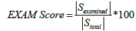
where Sexamined and Stotal are sets which contain the statements that are examined to localize the fault and the total number of executable statements present in the program respectively. For example, if we have a faulty program P and the EXAM Score of FL technique1 is lesser than FL technique2, then FL technique1 is more effective than FL technique 2.
Results Obtained
We present the effect of unique and slicing techniques when superimposed on Tarantula [21], Jaccard, Ochiai [6] and DStar [11] SBFL methods.
From (Table 2), we can observe that on applying the slicing technique the line of code executed are reduced to a great extend in all the seven siemens suite program cases. Hence by applying this technique our search space reduces which in turn reduces the cost and time of execution of the program.
| Program Name | No. of lines executed before slicing | No. of lines executed after slicing (Average) | % reduction in total no. of lines executed |
|---|---|---|---|
| tcas | 65 | 49 | 24.615 |
| totinfo | 122 | 59 | 51.639 |
| replace | 244 | 70 | 71.311 |
| Printtokens | 195 | 79 | 59.487 |
| Printtokens2 | 200 | 111 | 44.5 |
| Schedule | 152 | 106 | 30.263 |
| Schedule2 | 128 | 97 | 24.218 |
Table 2: Execution of the program.
So, from (Table 2) we can observe that by applying slicing technique we get an average 43.719% reduction in the total no. of lines executed.
From (Table 3) , it is clearly visible that on applying the unique technique we get rid of all the redundant test cases which do not contribute to any significant change in the ranking of the statements according to their suspiciousness, hence we are left with only relevant test cases. Thus, the time and cost of computation of suspiciousness score for different test cases is reduced significantly. The first column of this table describes the average number of passed test cases for all the versions of different siemens suite programs. The second column describes the average number of failed test cases for all the versions of different siemens suite programs. The third column describes the average number of passed test cases for all the versions of different siemens suite programs after unique technique is applied and lastly the fourth column describes the average number of failed test cases for all versions of different siemens suite programs after unique technique is applied.
| Program Name | Passed Test cases before unique (Average) | Failed Test Cases before unique (Average) | Passed test cases after unique (Average) | Failed test cases after unique (Average) |
|---|---|---|---|---|
| tcas | 1551 | 57 | 8 | 2 |
| totinfo | 943 | 81 | 138 | 33 |
| replace | 5476 | 66 | 1265 | 25 |
| Printtokens | 4076 | 76 | 1800 | 49 |
| Printtokens2 | 3900 | 218 | 1534 | 202 |
| Schedule | 2391 | 259 | 457 | 23 |
| Schedule2 | 2674 | 36 | 648 | 16 |
Table 3: Test cases after unique.
The (Table 4) shows a comparison between the total number of lines of code executed (if all the relevant versions of the seven siemens suite programs are included) in order to reach the buggy line before and after slicing in the best and the worst case scenarios.
| Method | % of statements executed in Best Case before Slicing | % of statements executed in Worst Case before slicing | % of statements executed in Best Case after slicing | % of statements executed in Worst Case after slicing |
|---|---|---|---|---|
| Tarantula | 14.304 | 20.817 | 8.414 | 15.235 |
| Jaccard | 13.488 | 20.048 | 8.414 | 15.235 |
| Ochiai | 11.011 | 17.551 | 8.414 | 15.235 |
| DStar | 11.312 | 18.428 | 8.153 | 15.215 |
Table 4: Statements executed in Worst Case after slicing.
From (Table 3), we observe that 15.87% statements are executed on an average by the SBFL methods before slicing, while only 11.79% statements need to be executed on an average by the SBFL methods after slicing.
The (Table 5) shows a comparison between the total number of lines of code executed (if all the relevant versions of the seven siemens suite programs are included) in order to reach the buggy line before and after the unique technique was applied in the best and the worst case Scenarios.
| Method | % of statements ececuted in Best Case before unique | % of statements executed in Worst Case before unique | % of statements executed in Best Rank after unique | % of statements executed in Worst Case after unique |
|---|---|---|---|---|
| Tarantula | 14.304 | 20.817 | 13.079 | 19.867 |
| Jaccard | 13.488 | 20.048 | 11.854 | 18.675 |
| Ochiai | 11.011 | 17.551 | 9.706 | 16.306 |
| DStar | 11.312 | 18.428 | 9.572 | 16.232 |
Table 5: Statements executed in Best Rank after unique.
From (Table 5), we observe that 15.87% statements are executed on an average by the SBFL methods before unique technique, while only 14.412% statements need to be executed on an average by the SBFL methods after unique technique.
The (Table 6) shows a comparison between the total number of lines of code executed (if all the relevant versions of the seven siemens suite programs are included) in order to reach the buggy line before and after both the unique and slicing technique were applied in the best and the worst-case scenarios.
| Method | % of statements executed in Best Case before unique slicing | % of statements executed in Worst Case before unique slicing | % of statements executed in Best Case after unique slicing | % of statements executed in Worst Case after unique slicing |
|---|---|---|---|---|
| Tarantula | 14.304 | 20.817 | 8.655 | 15.536 |
| Jaccard | 13.488 | 20.048 | 8.655 | 15.536 |
| Ochiai | 11.011 | 17.551 | 8.655 | 15.536 |
| DStar | 11.312 | 18.428 | 8.213 | 15.516 |
Table 6: SBFL methods before applying unique-slicing technique.
From (Table 6), we observe that 15.87% statements are executed on an average by the SBFL methods before applying unique-slicing technique, while only 12.038% statements need to be executed on an average by the SBFL methods after applying unique-slicing technique. Thus, from the above four results table it is quite clear that slicing technique enhances the effectiveness of the SBFL methods in the best way.
In this section we will further discuss upon the time taken by different SFL technique when unique and slicing techniques are applied on the siemens suite programs.
In (Table 7) we have calculated total time for all the relevant versions of all siemens suite programs).
| Method | Time taken without applying any technique (in seconds) | Time taken after applying unique technique (in seconds) | Time taken after applying slicing technique (in seconds) | Time taken after applying unique slicing technique (in seconds) |
|---|---|---|---|---|
| Tarantula | 21.017686 | 18.104703 | 6.964918 | 13.546188 |
| Jaccard | 20.946931 | 17.42287 | 5.940318 | 6.95054 |
| Ochiai | 21.190692 | 16.832766 | 5.374688 | 9.468757 |
| DStar | 27.614273 | 19.980458 | 5.405468 | 9.40428 |
Table 7: Calculated total time for all the relevant versions of all siemens suite programs.
From the above table it is clearly visible that our proposed techniques are quite time efficient. For the slicing technique we find that the time required for complete execution of SBFL methods for all the faulty versions reduces by 73.391% on an average. For unique technique the reduction in total execution time was observed as 19.723% while for unique-slicing technique it was observed as 55.907%. Thus, we can say out of the three techniques, slicing comes out to be most time efficient.
The graphical representation of our results has also been provided Figure 1.

Figure 1: Graphs of SBFL techniques.
The method Ochiai [6] is derived from the base method Tarantula [21], but it gives better results than Tarantula [21].
From the comparison graph of all the four SBFL methods we can observe that the slicing curve is above of all the remaining curves which shows that slicing enhances the effectiveness of a SBFL technique to the greatest. The unique-slicing technique curve overlaps approximately with the slicing curve, hence we can say that this technique offers approximately same effectiveness but is less time efficient as compared to slicing technique.
Related Work
Program bugs are located by some of the slicing based techniques. Weiser [13] proposed static slicing technique which is one of these.
The debugging search domain is reduced through the method of slicing and is based on the idea that a test case which failed due to an incorrect value stored in a variable at a statement, then that defect will be found in the static slice associated with that variable-statement pair. This means that instead of tracing the entire program [13] we only have to search in very limited region which is bounded by the slice. A program dice technique was developed by Lyle and Weiser in which the difference between sets of two groups of static slices was developed which further reduced the search domain for possible locations of a fault. Static slice-based fault localization methods were further improved by development of dynamic slicing and execution slicing. Debroy [22] proposed a grouping-based technique. This technique uses the strategy in which program components were grouped based on the number of failed tests that execute that component and ranks the group that contains components that have been executed by more failed tests. So, the grouping was done with group order as the first priority and suspiciousness as the second priority, which then computed by fault localization techniques. Then spectrum-based multiple fault localization was also introduced. Mayer and Stumptner [24] explained techniques which used source code to automatically generate program models. They proved that one of best accuracy providing model was generated by means of abstract interpretation [25]. So there are many Model-based approaches developed by Mayer, Wotawa, Stumptner, Yilmaz and Williams. Although modelbased approaches are generally used for multiple faults but they can be used for single fault case also which occurs during software debugging. The techniques developed from 1977 to November 2014 [23] were fully compiled and presented by Wong et al in a survey of fault localization [2]. In that survey he classified the techniques in eight categories: program slicing, spectrum-based, statistics, program state, machine learning, data mining, model-based debugging, and additional techniques. The latest tools developed for fault localization was also presented at their survey.
Conclusion
In this paper, we have presented the details of our slicing technique, unique technique as well as unique-slicing technique that are an assist in fault localization. Based on the results of executing a test suite for a faulty program, the slicing technique reduces the search space (as the total number of lines of code to be executed are reduced), the unique technique removes all the redundant test cases (only relevant test cases are executed) and lastly as the name suggests the unique slicing technique performs both the operations. To provide the visual mapping, different colours have been used on the plot to distinguish between the applied techniques. The results show that our technique is very effective as well as efficient for helping locate suspicious statements that may be faulty and suggest some directions for future work.
References
- Keijiro Araki, Zengo Furukawa, and Jingde Cheng. A general framework for debugging IEEE Software, 8(3):14–20, 1991.
- W. Eric Wong, Ruizhi Gao, Yihao Li, Rui Abreu, and Franz Wotawa- A Survey on Software Fault Localization.
- Thomas G. Evans and D. Lucille Darley. On-line debugging techniques: A survey. In Pro-ceedings of the Fall Joint Computer Conference, AFIPS’66 (Fall), pages 37–50, 1966.
- John T. Gilmore. Tx-o direct input utility system. Memo 6M-5097, 1957. Lincoln Laboratory, MIT.
- Thomas G. Stockham and Jack B. Dennis. Flit - flexowriter interrogation tape: A symbolic utility program for tx-o. Memo 5001-23, July 1960. Department of Electric Engineering, MIT.
- Naish L., Jie L. J., and Kotagiri R., A model for spectra-based software diagnosis. ACM Transactions on Software Engineering and methodology (TOSEM), 2011, 20(3), pp.1-32
- R. M. Balzer. Exdams: extendable debugging and monitoring system. In Proceedings of the
- Spring Joint Computer Conference, AFIPS’69 (Spring), pages 567–580, 1969. J. C. Munson and T. M. Khoshgoftaar, “The detection of fault-prone programs,”IEEE Trans. Softw. Eng., vol. 18, no. 5, pp. 423–433, May 1992.
- G. J. Pai and J. B. Dugan, “Empirical analysis of software fault content and fault proneness using Bayesian methods,” IEEE Trans. Softw. Eng., vol. 33, no. 10, pp. 675–686, Oct. 2007.
- C. S. Wright and T. A. Zia, “A quantitative analysis into the economics of correcting software bugs,” in Proc. Int. Conf. Comput. Intell. Security Inf. Syst., Torremolinos, Spain, Jun. 2011, pp. 198–205.
- Wong W. E., Debroy V., Gao R., and Li Y., The DStar method for effective software fault localization. IEEE Transactions on Reliability, 2016, 63(1), pp. 290-308. DOI: 10.1109/TR.2013.2285319
- M.Weiser. Program slicing. IEEE Transactions on Software Engineering, 10(4):352–357, 1984.
- M.Weiser. Programmers use slices when debugging. Communications of the ACM, 25(7):446– 452, 1982.
- J.R.Lyle and M.Weiser. Automatic program bug location by program slicing. In Proceedings of International Conference on Computers and Applications, pages 877–883, 1987.
- H.Agrawal and J.R.Horgan. Dynamic program slicing. In Proceedings of the ACM SIGPLAN Conference on Programming Language Design and Implementation, pages 246–256, 1990.
- H.Agrawal, R.A.DeMillo, and E.H.Spafford. Debugging with dynamic slicing and backtracking. Software – Practice Experience, 23(6):589–616, 1993.
- Zhang Z., Yan L., Qingping T., Xiaoguang M., Ping Z., and Xi C., Deep LearningBased Fault Localization with Contextual Information. IEICE Transactions on Information and Systems, 2017, 100(12), pp. 3027-3031.
- Wong W. E., Debroy V., Golden R., Xu X., and Thuraisingham B., Effective software fault localization using an RBF neural network. IEEE Transactions on Reliability, 2012, 61(1), pp. 149-169. DOI: 10.1109/TR.2011.2172031
- Wong W. E., and Qi Y., BP neural network-based effective fault localization. International Journal of Software Engineering and Knowledge Engineering, 2009, 19(4), pp. 573-597. DOI: 10.1142/S021819400900426X
- D. E. Rumelhart, G. E. Hinton, and R. J. Williams, “Learning representations by back-propagating errors,” Nature, vol. 323, no. 6088, pp. 533–536, 1986.
- Jones J. A., and Harrold M. J., Empirical Evaluation of the Tarantula Automatic Fault Localization Technique. In Proceedings of the 20th IEEE/ACM Conference on Automated Software Engineering, 2005, pp. 273-282, Long Beach, California, USA. DOI: 10.1145/1101908.1101949
- V. Debroy, W. Eric Wong, X. Xu and B. Choi, A grouping-based strategy to improve the effectiveness of fault localization techniques, in Proceedings of the 10th International Conference on Quality Software, Zhangjiajie, China, July 2010, pp. 13#22.
- W. Eric Wong, Ruizhi Gao, Yihao Li, Rui Abreu, and Franz Wotawa. A survey on software fault localization. IEEE Transactions on Software Engineering, 42(8):707–740, 2016.
- W. Mayer and M. Stumptner. Evaluating models for modelbased debugging. In Proceedings of International Conference on Automated Software Engineering (ASE’08).
- W. Mayer and M. Stumptner. Abstract interpretation of programs for model-based debugging. In Proceedings of International Joint Conference on Artificial Intelligence (IJCAI’07).
- https://man7.org/linux/man-pages/man1/gcov-tool.1.html
- Higor A. de Souza, Marcos L. Chaim, and Fabio Kon , Spectrum-based Software Fault Localization: A Survey of Techniques, Advances, and Challenges.