Spanish
  Chinese
  Russian
  German
  French
  Japanese
  Portuguese
  Hindi
Hindi Research Article, J Chem Appl Chem Eng Vol: 1 Issue: 2
A Uniform Nonlinearity Criterion Resulting from Normalization of Nonlinear Models Applied for Calibration Curve and Standard Addition Methods
Anna Maria MichaÅ‚owska-Kaczmarczyk1, Aneta Spórna-Kucab2 and Tadeusz MichaÅ‚owski2*
1Department of Oncology, The University Hospital in Cracow, 31-501 Cracow, Poland
2Department of Analytical Chemistry, Technical University of Cracow, 31-155 Cracow, Poland
*Corresponding Author : Tadeusz Michałowski
Faculty of Chemical Engineering and Technology, Cracow University of Technology, Warszawska 24, 31-155 Cracow, Poland
Tel: +48126282035
E-mail: michalot@o2.pl
Received: October 10, 2017 Accepted: October 23, 2017 Published: October 31, 2017
Citation: MichaÅ‚owska-Kaczmarczyk AM, Spórna-Kucab A, MichaÅ‚owski T (2017) A Uniform Nonlinearity Criterion Resulting from Normalization of Nonlinear Models Applied for Calibration Curve and Standard Addition Methods. J Chem Appl Chem Eng 1:2 doi:10.4172/2576-3954.1000108
Abstract
It is proved that the shape of equations obtained after transformation of real (x, y) into normalised (u, v) variables enables to present polynomial and rational functions in a unified form. In terms of normalised variables, the equations applicable for calibration curves are analogous to ones obtained for standard addition method. It enables to apply a common criterion adaptable for both methods of chemical analysis.
Keywords: Chemical analysis; Standard addition; Calibration; Non-linear models
Abbreviations
CCM: Calibration Curve Method; LSM: Least Squares Method; SAM: Standard Addition Method
Introduction
The instruments used in chemical laboratories require prior calibration before they are used to produce relevant analytical data. Calibration [1-8] is defined as the sequence of operations that enables to establish, under specified conditions, the functional relationship between values of the measurable signal y (output quantity, e.g. absorbance) indicated by a measuring device and the corresponding values of variable x (input quantity or property, e.g. concentration) realised by standards of an analyte X, under defined conditions assumed. If the calibration is performed incorrectly, the results of analyses will be unreliable [1,5].
We consider polynomial and rational, monotonically increasing functions y=y(x), i.e., dy/dx>0 within defined x-range. For the monotonic function y=y(x), there is an inverse relation x=x(y) within the specified y-range. The model y=y(x) will be applied to the set of arranged experimental data (xj, yj), j=1, ..., N, where yj ≤ yj+1 at xj ≤ xj+1.
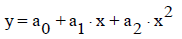
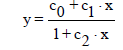
The linear relationship y=a+b⋅x is applicable only within a limited (narrowed down) range for x. For a more extended range of the variable x, the non-linear (parabolic, hyperbolic) models seem to be more adaptable. They are represented by equations:
 (1)
(1)
 (2)
(2)
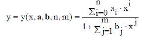
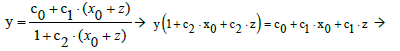
for parabola (1), and hyperbola (2). Equation 2 is a particular case of rational function [9,10]
 (3)
(3)
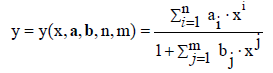
where a=[a0, ..., an]T, b=[b1, ..., bm]T, ai, bj ∈ ℜ. A particular case are there the functions of the Padé type [11-14]; some of them (with m=n+1) were applied [15] to semi-empirical modelling purposes. In a common opinion, rational functions have greater approximative power than polynomial functions – in the sense that, with the same number of parameters involved, they enable to get better approximation. The modified rational function (3) where a0=0, i.e.,
 (4)
(4)
is applicable for standard addition method [16,17].
Equations (1) and (2) assume linear form at a2 = c2 = 0. The model (2) and its simpler form, with c0 = 0, proved to be applicable in analyses made with use of AAS method [9] and in potentiometric acid-base titration curves, where generalised Simms constants [15,18,19] are involved.
Numerous examples testifying in favour of hyperbolic approximations are provided in [20-24] where the approximation
 (5)
(5)
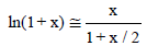
has been applied against the approximation
ln(1+ x) ≅ x (6)
referred to the Gran I method, and the approximation ln(1+x) ≅ x – x2/2. The validity of the approximations is clearly visible in Table 1, [22]. The divergences are, for example: 0.02% in Equation 6 and 2.5% in Equation 7 at x=0.05; 0.27% in Equation 6 and 9.8% in Equation 7 at x=0.20; 3.8% in Equation 6, and 44% in Equation 7 at x=1.00.
| 1 | x | 0.05000 | 0.10000 | 0.20000 | 0.25000 | 0.50000 | 0.75000 | 1.00000 |
| 2 | ln(1+x) | 0.04879 | 0.09531 | 0.18232 | 0.22314 | 0.40547 | 0.55962 | 0.69315 |
| 3 | x – x2/2 | 0.04875 | 0.09500 | 0.18000 | 0.21875 | 0.37500 | 0.46875 | 0.50000 |
| 4 | x/(1+x/2) | 0.04878 | 0.09524 | 0.18182 | 0.22222 | 0.40000 | 0.54545 | 0.66667 |
Table 1: The ln(1+x) values and their approximations.
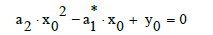
Standard addition method (SAM)
Let us introduce a new variable z, involved in relation
x=x0+z (7)
where x0 is the initial concentration of an analyte X in the sample tested. Let y0 be the signal related to x=x0 (i.e., z=z0=0) and N be the number of standard additions, i.e., N+1 experimental points {(zj, yj) | j=0,1, ..., N} are registered.
 (8)
(8)
where:
 (9)
(9)
 (10)
(10)
 (11)
(11)
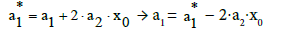
At a0=0 in Equation (9), from Equations (9)–(11) we have, by turns:
 (12)
(12)
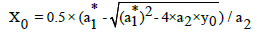 (13)
(13)
where  and a2 are determined from Equation (8), according to LSM.
From Equation (2) we have, by turns,
 (14)
(14)
where:
 (15)
(15)
Before application of the LSM, Equation (14) should be rewritten into the form
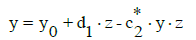 (16)
(16)
where:
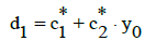 (17)
(17)
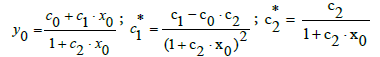
At c0=0, from Equation (15) we have, by turns,
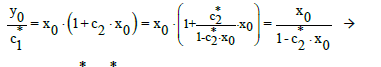
 (18)
(18)
and then from Equations (17) and (18) we have

Uniformity of Non-Linear Models
In order to compare the models applied within different ranges of concentrations and/or signals y registered, a uniformity (normality) procedure is necessary, i.e., both variables (x and y) should be normalised. Taking into account that nonlinear models are considered within different areas of chemical analysis, the resulting models should also be independent on the instrumental method applied for analytical purposes. The sensitivity of the method should also be considered. All the requirements are fulfilled when the normalised variables are introduced. The normalising procedure consists of two steps: (1°) calculation of parameters of the regression equation in its initial or transformed forms and (2°) formulation of the comparative criterion of fit of the modelling functions, in terms of normalised variables. The parameters of the functions are obtained by the least squares method (LSM). The functions considered will be related to the calibration curve and standard addition methods.
CCM
Let x1, ..., xN be the set of N ordered reference values and y1, ..., yN be their respective test values. Then for the arranged set of overdetermined experimental data (xj, yj), j=1,...,N (xj ≤ xj+1, yj ≤ yj+1), we introduce the relations:
 (20)
(20)
 (21)
(21)
where u ∈ <0,1>, v ∈ <0,1>. Applying Equations (20) and (21) in Equations (1) and (2), we get the formulas:
 (22)
(22)
 (23)
(23)
where: v = 0 for u = 0, and v = 1 for u = 1

and s=Δy/Δx is the mean sensitivity of the CCM; the s value is affected – to some degree – by the range <x1, xN> of the variable x chosen to plot the related calibration curve. The straight line connecting the points (0, 0) and (1, 1) in the co-ordinates (u, v) has the form
v=u (24)
SAM
Introducing:
 (25)
(25)
 (26)
(26)
into Equations (1) and (2), we have, in terms of normalised variables (w*, v*):
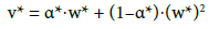 (27)
(27)
where v*=0 at w*=0 and v*=1 at w*=1. Applying Equations (25) and (26) in Equation 14, we have
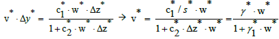 (28)
(28)
Assuming that the curve passes through the points (w*, v*) = (0, 0) and (1,1), we get γ1* =γ * −1, and then we have the relation
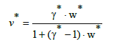 (29)
(29)
where: 

Some remarks
Note that the formulas for SAM with asterisked data (α*, γ*, s*, w* and v*) involve x0, not x1. The x1 enters the formulas for α, γ, s, u and v, referred to CCM. Similarities between the formulas: (22) and (27) or (23) and (29) are the basis for application of identical criteria for CCM and SAM; these formulas are in close relevance to the homotopy problem [25], considered within topology.
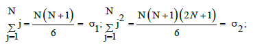
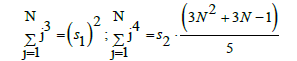
Applying equidistant values for zj, i.e., zj+1 – zj = Δz for j=0, ..., N-1, we get zj = (j/N)⋅Δz*. Similarly, at xj+1 – xj=Δx, for j=1, ..., N-1, we have xj = x1 + (j–1)/(N–1)⋅Δx. Then the external parameters of the corresponding regression equations can be calculated with use of the following formulas:
A nonlinearity criterion of the model
As the criterion of the nonlinearity one can assume the area between the lines (5)–(7) and straight line (Equation 8) in the normalised variables (u, v) [9] (Figure 1). This integral criterion is expressed by

Figure 1: The exemplary plot v=v(u) [9] and the line v=u (Equation 24).
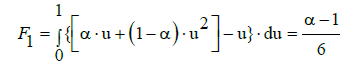 (31)
(31)
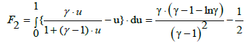 (32)
(32)
When referring to standard addition, the parameters α, β, γ should be replaced by α*, β*, γ*. Setting lnγ=ln (1+γ–1) and applying the approximation (5), from Equation (32) we get
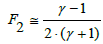 (33)
(33)
The area between the line v=v(u) and the line v=u, plotted in the normalized coordinates (u, v), is the measure of nonlinearity of any monotonic relationship obtained on the basis of experimental points (xj, yj)|j=1, ..., N}, compare with Figure 1. This area is expressed as follows
 (34)
(34)
More complex rational functions y=y(x) (Equations 3 and 4) were also considered in references [9,16,17], e.g. the function
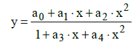 (35)
(35)
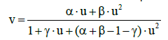
is expressed, in normalized variables, by the relation v=v(u)
 (36)
(36)
 (37)
(37)
For the function (36), illustrated by Figure 1, we have v ≥ u within u ∈< 0, 1 >.
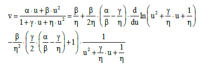
From the tables of elementary integrals [26,27] we find, among others,
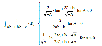 (38)
(38)
with Δ=b2 – 4ac. Setting a=1, b=γ/η, c=1/η and ξ=u in Equation (38), we get [9]
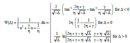 (39)
(39)
where
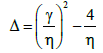 (40)
(40)
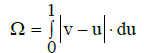
In particular, for Δ<0 we get the Ω value (Equation 34)
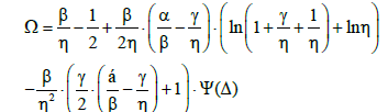 (41)
(41)
Final Comments
Calibration is one of the basic activities realized within any analytical measurement. On the step of calibration, the functional relationship between the y-values indicated by measuring instrument and concentrations x of the standard samples (s) is established under strictly defined conditions of the calibration procedure.
In univariate calibration, with x as an independent variable, the linear regression is most frequently used and abused [28]. In some instances, however, a nonlinear model expressing a functional relationship y=y(x) between variables x and y within defined x-range provides better description of a relationship between x and y, under specified conditions. To obtain a valid model, the analyst must also subjectively decide on the boundaries of the system and on the attributes to be quantified in the model.
The calibration enables, among others, to estimate the real value x0 of the measurand from the experimental value obtained in the measurement. The calibration provides an empirical relationship between the measured values.
The nonlinear modelling is done both for analytical and physicochemical purposes [2,29]. The success of calibration (accuracy, precision) depends on interrelations within the “triplet”: dataset {(xj, yj)|j=1, ..., N}, model y=y(x) and the analytical method applied. When applying the least squares method to linear regression, it is assumed that each data–point in a given x–range has a constant absolute variation (homoscedasticity). If y=y(x) is not a linear model with respect to changes in analyte concentration, i.e., y(x) cannot be sufficiently modelled by a first order polynomial, a nonlinear calibration model must be employed [29]. The nonlinear model is also necessary when the unknown sample contains some species affecting the y value; otherwise, the prediction will be inaccurate [30]. An accurate, univariate calibration is prohibited, in most cases, by matrix effects. In such instances, an issue is the standard addition method.
The uncertainty (errors) may also be the physical modifications (changes) taking place between the calibration and the measurement process using this curve. For example, if the temperature of the samples is not equal to the calibration temperature, then the results may be wrong. In flame AAS (FAAS), the change of temperature influences the surface tension of the liquid sample, and thus on the efficiency of nebulization preceding the sample atomization. The composition of the reference samples must be similar to the composition of the samples tested. This applies, in particular, to the sample matrix and the size of particles contained therein [31]. For example, analysis of blood serum samples for pesticide or drug residues should not be based on calibration curves based on measurement of signals for aqueous solutions of the respective reference substances [32]. Because the serum blood composition is not reproducible in calibration solutions, another method is required [33], especially the standard addition method.
In this work we have shown that for CCM, as an extrapolation method and for SAM, as the interpolation method, we obtain formally identical functional relations in a normalized, dimensionless system of coordinates. Hence results the possibility of applying a unified criterion of nonlinearity of the appropriate results of analysis. This criterion is independent of the scale and range of concentrations covered by the measurements, and the indications and sensitivity of the measuring devices.
References
- Danzer K, Currie LA (1998) Guidelines for calibration in analytical chemistry. Part I. Fundamentals and single component calibration (IUPAC Recommendations 1998). Pure Appl Chem 70: 993-1014.
- Curie LA (1999) Nomenclature in evaluation of analytical methods including detection and quantification capabilities: (IUPAC Recommendations 1995). Anal Chim Acta 391: 105-126.
- Müller MM (2000) Implementation of reference systems in laboratory medicine. Clin Chem 46: 1907-1909.
- May W, Parris R, Beck C, Fassett J, Greenberg R, et al. (2000) NIST Special Publication 260-136, Standard reference materials. Definitions of terms and modes used at NIST for value-assignment of reference materials for chemical measurements, U.S. Government Printing Office, Washington.
- Cuadros-RodrıÌÂÂÂguez L, Gámiz-Gracia L, Almansa-López E, Laso-Sánchez J (2001) Calibration in chemical measurement processes: I. A metrological approach. Trends Analyt Chem 20: 195-206.
- Jancke H, Malz F, Haesselbarth W (2005) Structure analytical methods for quantitative reference applications. Accred Qual Assur 10: 421-429.
- Åšwitajâ€ÂÂÂZawadka A, Konieczka P, Przyk E, NamieÅ›nik J (2005) Calibration in metrological approach. Analyt Lett 38: 353-376.
- Czichos H, Saito T, Smith L (2011) Handbook of metrology and testing, Springer-Verlag Berlin Heidelberg, Germany.
- Gorazda K, Michałowska-Kaczmarczyk AM, Asuero AG, Michałowski T (2013) Application of rational functions for standard addition method. Talanta 116: 927-930.
- Michałowski T, Pilarski B, Michałowska-Kaczmarczyk AM, Kukwa A (2014) A non-linearity criterion applied to the cali-bration curve method involved with ion-selective electrodes. Talanta 124: 36-42.
- Michałowski T, Rokosz A, Tomsia A (1987) Determination of basic impurities in mixtures of hydrolysable salts. Analyst 112: 1739-1741.
- Michałowski T (1988) Possibilities of application of some new algorithms for standardization purposes. Standardization of sodium hydroxide against commercial potassium hydrogen phthalate. Analyst 113: 833-835.
- MichaÅ‚owski T, Rokosz A, Negrusz-SzczÄ™sna E (1988) Use of Padé¸ approximants in the processing of pH titration data. Determination of the parameters involved in the titration of acetic acid. Analyst 113: 969-972.
- MichaÅ‚owski T, Rokosz A, KoÅ›cielniak P, ÅÂÂÂagan M, Mrozek J (1989) Calculation of concentrations of hydrochloric and citric acids together in a mixture with hydrolysable salts. Analyst 114: 1689-1692.
- Michałowska-Kaczmarczyk AM, Michałowski T (2016) Application of Simms constants in modeling the titrimetric analyses of fulvic acids and their complexes with metal ions. J Solution Chem 45: 200-220.
- Michałowska-Kaczmarczyk AM, Asuero AG, Martin J, Alonso E, Michałowski T, et al. (2014) A uniform nonline-arity criterion for rational functions applied to calibration curve and standard addition methods. Talanta 130: 307-314.
- Michałowski T, Pilarski B, Ponikvar-Svet M, Asuero AG, Kukwa A, et al. (2011) New methods applicable for calibration of indicator electrodes. Talanta 83: 1530-1537.
- Michałowski T (1992) Some new algorithms applicable to potentiometric titration in acid-base systems. Talanta 39: 1127-1137.
- Michałowski T, Gibas E (1994) Applicability of new algorithms for determination of acids, bases, salts and their mixtures. Talanta 41: 1311-1317.
- Michałowski T, Stępak R (1985) Evaluation of the equivalence point in potentiometric titrations with application to traces of chloride. Anal Chim Acta 172: 207-214.
- Michałowski T, Baterowicz A, Madej A, Kochana J (2001) Extended Gran method and its applicability for simultaneous determination of Fe(II) and Fe(III). Anal Chim Acta 442: 287-293.
- Michałowski T, Toporek M, Rymanowski M (2005) Overview on the Gran and other linearization methods applied in titrimetric analyses. Talanta 65: 1241-1253.
- Michałowski T, Kupiec K, Rymanowski M (2008) Numerical analysis of the Gran methods. A comparative study. Anal Chim Acta 606: 172-183.
- Ponikvar M, Michałowski T, Kupiec K, Wybraniec S, Rymanowski M (2008) Experimental verification of the modified Gran methods applicable to redox systems. Anal Chim Acta 628: 181-189.
- Homotopy groups of spheres.
- Piłat B, Wasilewski MJ (1985) Tables of integrals (in Polish), WNT Warsaw, 28.
- Table of Basic Integrals.
- Meloun M, Militky J, Kupka K, Brereton RG (2002) The effect of influential data, model and method on the precision of univariate calibration. Talanta 57: 721-740.
- Brauner N, Shacham M (1998) Identifying and removing sources of imprecision in polynomial regression. Math Comput Simul 48: 75-91.
- Booksh KS, Kowalski BS (1997) Calibration method choice by comparison of model basis functions to the theoretical in-strument response function. Anal Chim Acta 348: 1-9.
- Bouveresse E, Massart DL (1996) Standardization of near-infrared spectrometric instruments : a review. Vib Spectrosc 11: 3-15.
- Fagelj A, Parkany M (eds) (1999) The use of matrix reference materials in environmental analytical processes, The Royal Society of Chemistry, Cambridge, UK.
- De Noord OE (1994) Multivariate calibration standardization. Chemometr Intell Lab Syst 25: 85-97.