Spanish
  Chinese
  Russian
  German
  French
  Japanese
  Portuguese
  Hindi
Hindi Research Article, J Comput Eng Inf Technol Vol: 6 Issue: 4
Analytical Solutions of Heat Problems for Efficient Heat Transfer in a Nanofluid
Chaharborj SS1,2* and Yaghoub Mahmoudi3
1School of Mathematics and Statistics, Carleton University, Ottawa, Canada
2Department of Mathematics, Islamic Azad University, Bushehr Branch, Bushehr, Iran
3Department of Mathematics, Tabriz Branch, Islamic Azad University, Tabriz, Iran
*Corresponding Author : Sarkhosh S
Chaharborj, School of Mathematics and Statistics, Carleton University, Ottawa, Canada
E-mail: sseddighi2014@yahoo.com.my
Received: May 10, 2017 Accepted: June 15, 2017 Published: June 19, 2017
Citation: Chaharborj SS, Mahmoudi Y (2017) Analytical Solutions of Heat Problems for Efficient Heat Transfer in a Nanofluid. J Comput Eng Inf Technol 6:3. doi: 10.4172/2324-9307.1000179
Abstract
To find the approximate solutions of heat equations in a boundary layer flow, beneath a uniform free stream permeable continuous moving surface in a nanofluid is the main purpose of this paper. First, we will propose a neural network coupled with the Chebyshev polynomials. We will then study the heat transfer and heat flow equations by using the presented Chebyshev neural network. As it turns out, this method can obtain the approximate solutions for any kind heat transfer and heat flow equations.
Approximate answers can be more helpful to study the behavior of heat transfer heat flow, and it can ensure a more efficient heat transfer with a lower operational cost. The missing slopes f rr(0) and gr(0), for some values of the governing parameters, namely the nano-particle volume fraction φ, the mov- ing parameter λ and the suction/injection parameter f0 are determined using the proposed method. The obtained results of this method have been compared with other papers results of different methods.
Keywords: Heat transfer; Heat flow; Moving surface; Nano-fluid; Chebyshev neural network
Introduction
The boundary layer flow problems have various applications in the fluid mechanics. Most researchers have used the semi-analytical and numerical methods such as Runge-Kutta methods [1], finite difference methods [2], finite element methods [3] and spectral methods [4] to solve this type of equations. In recent years, for solving nonlinear differential equations, several analytical and semi-analytical methods have been established such as, variational iteration method [5,6], Adomian decomposition method [7], differential transform method [8], homotopy analysis method [9-13], and the spectralhomotopy analysis [14,15] and more recently, successive linearization method [16,17].
All analytical and semi-analytical methods mostly focus on the single and independent linear and non- linear equations of the boundary layer flow problems. In this paper we present an improved Chebyshev neural network method to solve the system of boundary layer problems. The considered system con- tains the nonlinear boundary differential equations governed from partial differential equations of heat equations in a boundary layer flow, beneath a uniform free stream permeable continuous moving surface in a nanofluid. Five various types elements, namely Ag, Cu, CuO, TiO2 and Al2O3 are examined as potential nanoparticles in a water-based fluid in [18,19], whereby their performance in the boundary layer flow over a permeable continuous moving surface with suction and injection are analyzed. Additionally, the parameters influencing the process’s fluid velocity, temperature and particle concentration are analyzed and discussed in detail.
Formulation of problem
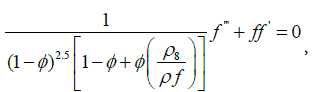
The flow model and coordinate system of a flat surface moving at a constant velocity uw in a par- allel direction to a free stream of a nanofluid of uniform velocity u∞ are shown in Figure 1. The dimensionless boundary layer equations of this model can be defined as follows [18-21],

Figure 1: Physical model and coordinate system; (a): flat plate moving out of the origin; (b): flat plate moving into the origin.
 (1)
(1)
 (2)
(2)
 (3)
(3)
 (4)
(4)
 (5)
(5)
With the boundary conditions as follows,


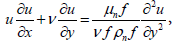
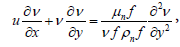
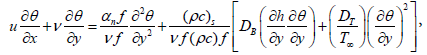
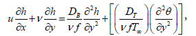
Here vw represents injection, suction and impermeable surface when vw>0, vw<0 and vw=0, respectively. Moreover, u and v are the velocity components along the x and y axes, respectively; T is the temperature of the nanofluid, μnf is the dynamic of the nanofluid, αnf is the thermal diffusivity of the nanofluid and ρnf is the density of the nanofluid, written as follows,
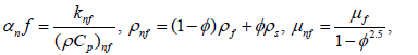
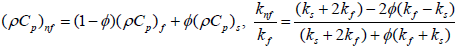 (6)
(6)
The equation of continuity is satisfied if a stream function Ψ(x, y) is chosen, such that,
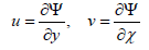 (7)
(7)
The similarly transformed equations is then introduced as follows,
 (8)
(8)
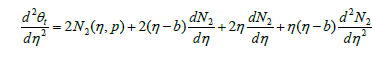
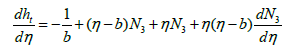
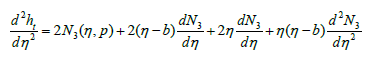
The governing equations (1) up to (5) are then transformed to the ordinary differential equations by
using the similarity transformation quantities as follows,
 (9)
(9)
 (10)
(10)
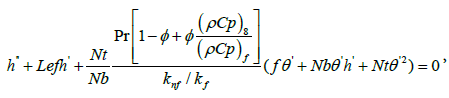 (11)
(11)
where the governing parameters Pr, Le, Nb and Nt are defined as follows,
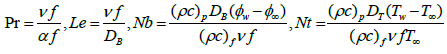 (12)
(12)
The transformed body conditions are given by,
 (13)
(13)
The skin friction coefficient and the Nusselt numbers are individually defined as,
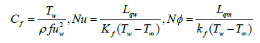 (14)
(14)
Where qw and qm are the surface heat flux and Tw is the surface shear stress, which are given by
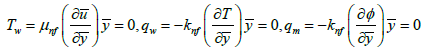 (15)
(15)
Substituting equations (6) and (8) into equation (14) and using the equation (15), we ge
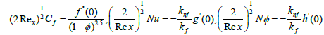 (16)
(16)
Structure of Chebyshev Neural Network
The structure of the network with the first m Chebyshev polynomial and single input and output layer are shown in Figure 2. In this network input data is extended to several terms using Chebyshev polynomials.

Figure 2: Structure of single layer Chebyshev Neural Network.
The learning algorithm can be used to update the network parameters and minimizing the error function. The weights of the proposed neural network can be to updated by using the error back propagation algorithm [22-25]. The network output with input data η and weight parameters, w, can obtain as follows,
Ni(η,w) = F(zi) , (17)
where F(zi)=zi is an active function and zi is a sum of the weighted expanded input data’s as follows,
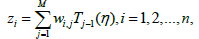 (18)
(18)
where η is the input data’s, Tj−1 and wi,j with j=1, 2, ..., M denotes the the Chebyshev polynomials and the weight vector, respectively. For updating the network weights we will use the principle of back propagation
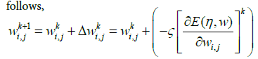 (19)
(19)
where ζ, k and E(η,w) are the learning parameter, iteration step and the error function, respectively. This parameters are using to update the network weights (Figure 2).
Chebyshev Polynomials
The Chebyshev polynomials of the first kind of degree n can be define as follows,
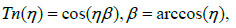 (20)
(20)
Which are orthogonal with respect to the weight function
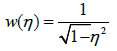
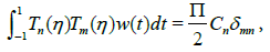 (21)
(21)
where, δnm is the Kronecker delta function and
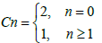 (22)
(22)
The first two Chebyshev polynomials are, T0(x) = 1 and T1(x) = x. The higher order Chebyshev
polynomials may be evaluated by the following formula,
Tn+1(x) = 2xTn(x) − Tn−1(x), (23)
where Tn(x) denotes the nth order Chebyshev polynomial
Chebyshev Neural Network Formulation for Heat Equations
The general formulation of the boundary value problems by using the neural network can be define as follows,
 (24)
(24)
where Ψi is the function which presents the structure of the boundary value equations. The parameters yi and ∇ are showing the solution and differential operators, respectively. If yi,t(η, w) are defined the trial solutions, then the equation (24) can be rewrite as,
 (25)
(25)
Therefore, the minimization equation [22,23,24] of the equation (25) can be shown as the following form,
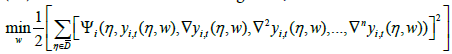 (26)
(26)
Trial solutions of the equations (9) up to (11) with the input parameter η and unknown weight parameter
w is written as follows,
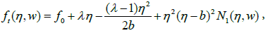 (27)
(27)
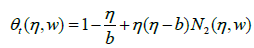 (28)
(28)
.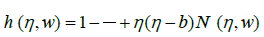 (29)
(29)
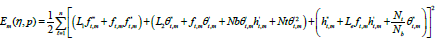
with, η ∈ [0, b]. The general form of the error function for the equations (9) up to (11) is given by,
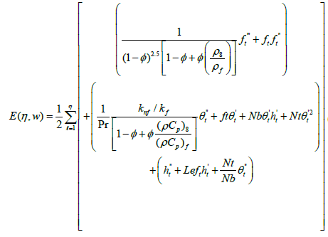 (30)
(30)
For minimizing the proposed error function corresponding to the input data’s, η, gradient of the error function with respect to the unknown parameters w will be used.
Computation of gradient for optimizing the weight values
As seen from the equations (30), this function is involve to function N (η, w) and derivatives of this function. Therefore, we need to obtain the derivative of this function with respect to the inputs parameters η as follows,
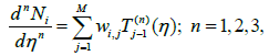 (31)
(31)
where wi,j denotes the network parameters and Tj-1 denote the first, second and third derivatives of (n) the Chebyshev polynomials for n=1,2,3 respectively. Therefore, the equations (27) up to (29) can be rewritten as follows,
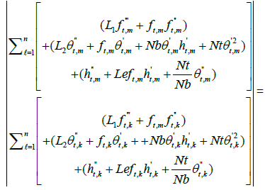
Now, for minimizing the error function (30), the gradient of this function with respect to the parameters wi,j are given by,
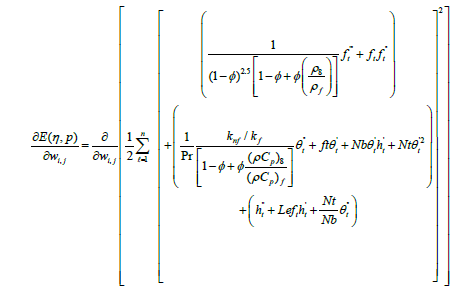 (32)
(32)
Finally, approximate solutions for the proposed heat equations can be computed by using the converged Cheby-shev neural network results in the equations (27) up to (29).
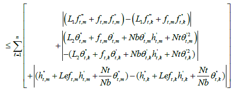
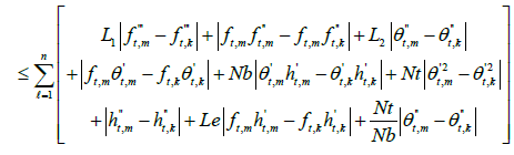
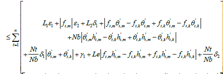
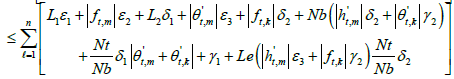
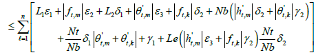
Convergence of the error function
In this section we investigate the convergence analysis of error function. Let Em(η, p) be a sequence of error functions as follows,
 (33)
(33)
then, sequence Em(η, p) converges uniformly to a function E(η, p) if and only if for every c>0 there exists an N so that m>N and k>N implying that |Em(η, p)−Ek(η, p)|<c. Some sufficient conditions for the convergence are as follows,
A1:  are uniformly convergence for η ∈R
A2: 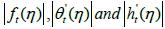 are uniformly bounded for η ∈R . For
 we have,
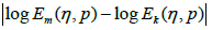
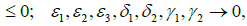
 This mean that
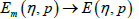 when
when 
Numerical Simulations
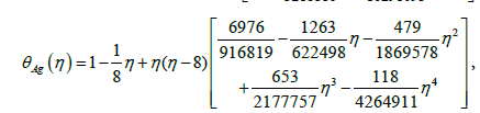
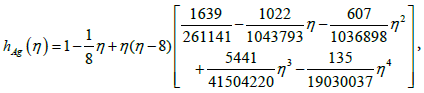
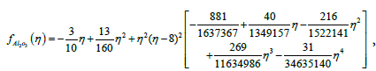
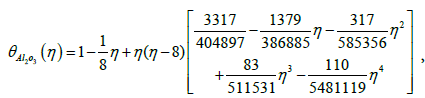
The analytical solutions of the nonlinear heat equations (9) up to (11) by using the proposed method with the five Chebyshev polynomials can be shown as follows,
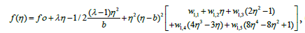 (34)
(34)
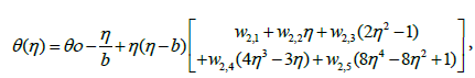 (35)
(35)
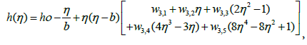 (36)
(36)
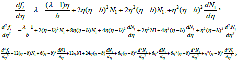
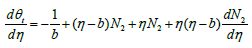
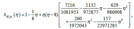
After substituting the updated weights, wi,j , (i-1,2,3; j=1,…,5) in the equations (34) up to (36), the analytical approximations of
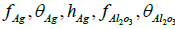 and
and  can be obtained as follows,
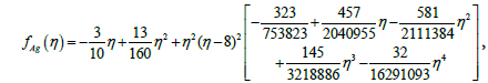 (37)
(37)
 (38)
(38)
 (39)
(39)
 (40)
(40)
 (41)
(41)
 (42)
(42)
Results and Discussion
Approximate solutions of the nonlinear ordinary differential equations (9) up to (11) with the boundary conditions (13) were obtained by using the proposed Chebyshev neural network
method. The missing slopes f(0)tt and g(0)t, for some values of the governing parameters, namely the nanoparticle volume fraction φ, the mov- ing parameter λ and the suction/injection parameter f0 are determined by using the Maple, Matlab softwares coupled with the Chebyshev neural network method.
Five types of nanoparticles were studied, namely, Silver Ag, Copper Cu, Copper Oxide CuO, Titania TiO2 and Alumina Al2O3 as shown in the Table 1 [19,20]. The volume fraction of nanoparticles is from 0 to 0.2 (0 ≤ φ ≤ 0.2) in which φ=0 corresponds to the regular Newtonian fluid. The numerical results are summarized in the Tables 2 and 3 and Figures 3-14. Figures 3-8 are showing the variation of f(0) tt (skin-friction coefficient) with λ for the water nanoparticles Ag, Cu, CuO, TiO2 and Al2O3 and different values of f0 when Nt=0.1, Nb=0.3, Le=1, Pr=0.1 and φ=0.1. It is seen that the solution is unique when λ ≥ 1, while dual solutions are found to exist when 0 ≤ λ ≤ 1 and trinal solutions are found when λ ≤ 0.
| Physical roperties/Nanoparticles | ρ (Kgm-3) | Cρ (Jkg-1 K-1) | k (Wm-1 K-1) | β×105 (K-1) |
|---|---|---|---|---|
| H2O | 997.1 | 4179 | 0.613 | 21 |
| Au | 10500 | 235 | 429 | 1.89 |
| Cu | 8933 | 385 | 401 | 1.167 |
| CuO | 6320 | 531.8 | 76.5 | 1.8 |
| Al2O3 | 3970 | 765 | 40 | 0.85 |
| TiO3 | 4550 | 686.2 | 8.9538 | 0.9 |
Table 1: Thermophysical properties of water and nanoparticles [19,20].
| F0 | λc | ||
|---|---|---|---|
| Weidman et al. [25] | Pop et al. [18] | ChNN | |
| -0.50 | -0.1035 | -0.1035 | -0.1034 |
| -0.25 | -0.2125 | -0.2181 | -0.2124 |
| 0.00 | -0.3541 | -0.3541 | -0.3540 |
| 0.25 | -0.5224 | -0.5227 | -0.5222 |
| 0.50 | -0.7200 | -0.7202 | -0.7200 |
Table 2: Comparison of λc for various f0 when φ=0 (purefluid).
| Physical Properties/F0 | λc | ||||
|---|---|---|---|---|---|
| Ag | Cu | CuO | TiO3 | Al2O3 | |
| -0.3 | -0.1590 | -0.1660 | -0.1929 | -0.1929 | -0.1955 |
| 0.3 | -0.6115 | -0.5997 | -0.5817 | -0.1519 | -0.5595 |
Table 3: Values of λc for different nanoparticles and different values of f0 when φ=0.1.

Figure 3: Variation of the reduced skin-friction coefficient f (0)tt with λ for φ = 0.

Figure 4: Variation of the reduced skin-friction coefficient f(0)tt with λ for Ag-water nanoparticale.

Figure 5: Variation of the reduced skin-friction coefficient f(0)tt with λ for Cu-water nanoparticale.

Figure 6: Variation of the reduced skin-friction coefficient f(0)tt with λ for CuO-water nanoparticale

Figure 7: Variation of the reduced skin-friction coefficient f(0)tt with λ for TiO2-water nanoparticale.

Figure 8: Variation of the reduced skin-friction coefficient f(0)tt with λ for Al2O3-water nanoparticale.

Figure 9: Variation of −θt(0) with λ for Ag-water nanoparticale.

Figure 10: Variation of −θt(0) with λ for Al2O3-water nanoparticale.

Figure 11: Velocity profile for Ag-water nanofluid.

Figure 12: Velocity profile for Al2O3-water nanofluid.

Figure 13: Temperature profiles for Ag-water nanofluid

Figure 14: Temperature profiles for Al2O3 water nanofluids.
As seen from these figures the values of f(0)tt are positive when λ ≤ 0. They become negatives when λ ≥ 1 and positive-negative when 0 ≤ λ ≤ 1 for all values of the suction/injection parameter f0. The Chebyshev neural network can give also third solutions for f(0) ttwhen λ ≤ 0. The third solution is coupled with the second solution as shown in Figures 3-8. Physically, a positive value of f(0)tt means that the fluid exerts a drag force on the plate, and a negative value means the opposite. The zero value of f(0)ttwhen λ=1 does not mean separation, but it corresponds to the equal velocity of the plate and the free stream.
Figures 9 and 10 show the variation of −gt(0) with λ for Ag and Al2O3-water nanofluid and different values of f0 when Nt=0.1, Nb=0.3, Le=1, Pr=0.1 and φ=0.1. By using the fifth order Runge- Kutta method with shooting technique can find dual solution for −gt(0). The Chebyshev neural network can give third solutions for -gt(0) which is couple with first solution as showed in Figures 9 and Figure 10. It is seen that the solution is dual when λ ≥ 0, while trinal solutions are found to exist when λ ≤ 0. The values of −gt(0) are positive for all values of λ, for all values of the suction/injection parameter f0.
Figures 3-10 are indicating that for a particular value of f0, the solution exists up to a certain critical value of λ, say λc. At this value, the boundary layer approximations break down, and thus the numerical solution cannot be obtained. The value λ=λc denotes a critical value of parameter λ and boundary layer will separate from the surface at value λc. The critical values of the parameter λc are showed in the Table 2, which shows a desirable
agreement with the previous investigations for the case f0=0. Moreover, from the table (2), we find that for all nanoparticles the values of |λc| increase as f0 increases. Therefore, suction delays the boundary layer separation, while injection accelerates it.
Figures 11 and 14 are presenting the velocity profile f(η)t and the temperature profile g(η) for the water nanofluids Ag and Al2O3 when Nt=0.1, Nb=0.3, Le=1, Pr=0.1, φ = 0.1, λ=-0.3 and f0=0, respectively.
For plotting these figures the equations (37) up to (42) have been used. It appears that all these profiles satisfied asymptotically the far field boundary conditions equation (13). The existence of triple solutions in the Figures 3-10 can be satisfied by the velocity and temperature profiles are showed in the Figures 11-14. The velocity profiles for the first, second and third solutions when λ=-0.3 shows that the velocity gradient at the surface is positive, which produces a positive value of the skin friction coefficient (Figures 13 and 14).
Conclusion
We have investigated the modified Chebyshev neural network for solving a complicated nonlinear dynamical heat system in a boundary layer flow, beneath a uniform free stream permeable continuous moving surface in a nanofluid. Numerical results show the effectiveness of our proposed method for solving complicated linear and nonlinear dynamical systems in the heat transfer and heat flow problems.
List of Symbols
cp specific heat capacity at constant pressure
Cf skin friction coefficient
f dimensionless stream function
k thermal conductivity
Nux local Nusselt number
Pr Prandtl number
qw surface heat flux
Rex local Reynolds number
Tw plate temperature
T fluid temperature
T∞ ambient temperature
u, v velocity components along the x and y directions, respectively
x, y Cartesian coordinates
Uw plate velocity
U∞ free stream velocity
Greek symbols
α thermal diffusivity
φ nonoparticle volume fraction
μ dynamic viscosity
θ dimensionless temperature
λ velocity ratio parameter
ν kinematic viscosity
Ψ stream function
τw surface shear stress
η similarity variable
Subscripts
s solid
f fluid
nf nanofluid
∞ ambient condition
w condition at the surface of the plate
Superscript
t differential with respect to
References
- Chaharborj SS, Kiai SS, Bakar MA, Ziaeian I, Fudziah I (2012) New impulsional potential for a paul ion trap. Int J Mass Spectrom 309: 63-69.
- Nayak I, Nayak AK, Padhy S (2016) Implicit finite difference solution for the magnetohydro–dynamic unsteady free convective flow and heat transfer of a third grade fluid past a porous vertical plate. IJMMNO 7: 4-19.
- John V (2016) Finite element methods for incompressible flow problems. Springer, Berlin.
- Chen S, Wang YA (2016) A Rational spectral collocation method for third-order singularly perturbed problems. J Comput Appl Math 307: 93-105.
- Moameni A (2011) Non-convex self-dual lagrangians New variational principles of symmetric boundary value problems. J Funct Anal 260: 2674-2715.
- Wazwaz AM (2016) Solving systems of fourth-order emden–fowler type equations by the variational iteration method. Chem Eng Commun 203: 1081-1092.
- Hosseini S, Babolian E, Abbasbandy S (2016) A new algorithm for solving van der pol equation based on piecewise spectral a domian decomposition method. IJIM 8: 177-184.
- Fidanoglu M, Komurgoz G, Ozkol I (2016) Heat transfer analysis of fins with spine geometry using differential transform method. IJMERR 5: 67-71.
- Shahlaei-Far S, Nabarrete A, Balthazar JM (2016) Homotopy analysis of a forced nonlinear beam model with quadratic and cubic nonlinearities. JTAM 54: 1219-1230.
- Semary MS, Hassan HN (2016) The homotopy analysis method for q-difference equations. ASEJ 1-7.
- Hayat T, Mumtaz M, Shafiq A, Alsaedi A (2017) Stratified magnetohydrodynamic flow of tangent hyperbolic nanofluid induced by inclined sheet. Applied Mathematics and Mechanics 38: 271-288.
- Zhu J, Wang S, Zheng L, Zhang X (2017) Heat transfer of nanofluids considering nanoparticle migration and second-order slip velocity. Appl Math Mech 38: 125-136.
- Zhao Q, Xu H, Tao L, Raees A, Sun Q (2016) Three dimensional free bio-convection of nanofluid near stagnation point on general curved isothermal surface. Appl Math Mech 37: 417-432.
- Motsa SS, Marewo GT, Sibanda P, Shateyi S (2011) An improved spectral homotopy analysis method for solving boundary layer problems. Boundary Value Problems 3-11.
- Rashidi MM, Rostami B, Freidoonimehr N, Abbasbandy S (2014) Free convective heat and mass transfer for MHD fluid flow over a permeable vertical stretching sheet in the presence of the radiation and buoyancy effects. ASEJ 5: 901-912.
- Bhatti MM, Shahid A, Rashidi MM (2016) Numerical simulation of fluid flow over a shrinking porous sheet by Successive linearization method. AEJ 55: 51-56
- Ahmed MAM, Mohammed ME, Khidir AA (2015) On linearization method to MHD boundary layer convective heat transfer with low pressure gradient. Propulsion and Power Research 4: 105-113.
- Pop I, Seddighi S, Bachok N, Ismail F (2014) Boundary layer flow beneath a uniform free stream permeable continuous moving surface in a nanofluid. JHMTR 1: 55-65.
- Alloui Z, Vasseur P, Reggio M (2011) Natural convection of nanofluids in a shallow cavity heated from below. IJTS 50: 385-393.
- Oztop HF, Abu-Nada E (2008) Numerical study of natural convection in partially heated rectangular enclo- sures filled with nanofluids. Int J heat and fluid flow 29: 1326-1336.
- Shah SD (2010) Heat Transfer in a Nanofluid Flow Past a Permeable Continuous Moving Surface.
- Mall S, Chakraverty S (2014) Chebyshev neural network based model for solving Lane Emden type equations. Appl Math Comput 247: 100-114.
- Mall S, Chakraverty S (2015) Numerical solution of nonlinear singular initial value problems of Emden Fowler type using Chebyshev Neural Network method. Neurocomputing 149: 975-982.
- Chaharborj SS, Chaharborj SS, Mahmoudi Y (2017) Study of Fractional Order Integro-Differential Equations by using Chebyshev Neural Network. J Math Statistics 13: 1-13.
- Weidman PD, Kubitschek DG, Davis AMJ (2006) The effect of transpiration on self-similar boundary layer flow over moving surfaces. IJES 44: 730-737.