Spanish
  Chinese
  Russian
  German
  French
  Japanese
  Portuguese
  Hindi
Hindi Research Article, J Appl Bioinforma Comput Biol Vol: 14 Issue: 1
Ant Target Algorithm: A Novel DNA Target Assembling Technique Using Optimized Graph and Ant Colony Optimization
Susobhan Baidya1, Sankhayan Choudhury2 and Rajat Kumar De3*
1Department of Computer Science and Engineering, Heritage Institute of Technology, Kolkata, India
2Department of Computer Science and Engineering, University of Calcutta, Kolkata, India
3Machine Intelligence Unit, Indian Statistical Institute, Kolkata, India
*Corresponding Author: Rajat Kumar De
Machine Intelligence Unit, Indian Statistical Institute, Kolkata, India
E-mail: rajat@isical.ac.in
Received date: 27 November, 2024, Manuscript No. JABCB-24-153424; Editor assigned date: 30 November, 2024, PreQC No. JABCB-24-153424 (PQ); Reviewed date: 14 December, 2024, QC No. JABCB-24-153424; Revised date: 09 April, 2025, Manuscript No. JABCB-24-153424 (R); Published date: 16 April, 2025, DOI: 10.4172/2329-9533.1000299.
Citation: Baidya S, Choudhury S, De RK (2025) Ant Target Algorithm: A Novel DNA Target Assembling Technique Using Optimized Graph and Ant Colony Optimization. J Appl Bioinforma Comput Biol 14:1.
Abstract
Target genome reassembling technique allows us to analyze specific regions of DNA, which facilitates clinical correction or disease detection. Here we have developed a methodology that focuses on the target region or region of interest. We have introduced a new methodology, called Ant-Target Algorithm (ATA), for target genome assembling using Ant Colony Optimization (ACO) and optimized graph, where we have used only the reads of the original sequence which has a length up to 109 bp. A section of reads are aligned to the reference target location and the remaining reads are rejected. Later aligned reads are stitched and reassembled. We have considered data sequence from NCBI and Ensembl BioMart, which have been obtained from organisms, like human, mouse, cat, zebrafish, dog, chimpanzee, lion, tiger, monkey, tortoise, camel, chicken, goat, duck, crow, Budgerigar bird, Atlantic salmon fish, blue whale, catfish and COVID virus. ATA has reported a maximum average error of 0.1% per sample, whereas existing technologies have reported an error of >0.1%.
Keywords: NP complete; Target genome assembling; Ant Target Algorithm (ATA); Ant Colony Optimization (ACO); Reads; Alignment
Keywords
NP complete; Target genome assembling; Ant Target Algorithm (ATA); Ant Colony Optimization (ACO); Reads; Alignment
Introduction
DNA reassembling is an NP-complete problem, we need to maintain a heavy graph to reconstruct the entire DNA from the reads. DNA sequencing techniques determine the order of nucleotides (A, C, T, G) in an unknown DNA chain. DNA sequence determines the flow of properties from ancestor to descendant. Due to the unavailability of appropriate technology, we are not able to read the nucleotide serially from the DNA strand. In Next Generation Sequencing (NGS) technology, DNA is sliced through chemical processes. The slices are termed as reads (100 bp-500 bp). The reads are then reassembled using some computational methods to recreate the original DNA. DNA reassembling technique needs a high level of computations and high memory storage [1].
Targeted Genome Sequencing (TS) is an approach sequencing, where we focus on of interest regions instead of the entire genome. TS is a functional tool for studying precise changes in the DNA sequence of an organism. A focused region contains a genetic region that has known relations with the disease under study. NGS technology offers speed, scalability and resolution to understand targeted genes of interest. Multiple genes can be studied in parallel. TS also yields a smaller, more manageable data set compared to whole-genome sequencing, making investigation easier. The existing Technologies- Whole Genome Sequencing (WGS) and Targeted Genome Sequencing (TS) have reported to have yielded more than 0.1% error. Targeted Genome Sequencing (TS) needs to prepare a targeted panel. It amplifies the targeted regions using amplicon/hybridization. There are so many commercially available Targeted Genome Sequencing (TS) platforms which are provided in Table 1. These target sequence panels are very costly and need amplicon enrichment/hybridization techniques. After sequencing, the next job is to assemble the reads and reconstruct the original genome [2].
A new algorithm for accurate assembling using long reads has been developed using ReFHap and DGS algorithms, where the researcher have used the long reads of PacBio HiFi and nanopore sequencing. They have the highest Genome fraction of 99.971%. Genome fraction is the total number of aligned bases in the reference, divided by the genome size. A linear time complexity de novo long reads genome assembly has been developed using GoldRush algorithm. It is a combination of GoldPath, GoldPolish, Tigmint-long and GoldChain. The algorithm is tested on Oxford nanopore sequencing reads. The algorithm has reached 99% base accuracy. Accurate long-read de novo assembly algorithm has been developed with Inspector. It has used long reads of PacBio CLR, PacBio HiFi and Oxford nanopore. The researchers have used five standard state-of-the-art assemblers Canu, Flye, wtdbg2, hifiasm and Shasta. They have reported 99.38% Mapping Ratio (MR) which is the maximum. IonTorrent and Min-ION sequencing methods are hybridized in an algorithm for an accurate complete genome sequence of clinical pathogens. This de novo assembly algorithm uses short reads of IonTorrent and long reads of MinIon. Here, some assemblers like, AssemblerSPAdes, Minimap +Miniasm+Racon (Hybrid assembler), Canu+unicycler (Hybrid assembler) and Canu+unicycler+pilonX3 (Hybrid assembler) have been used. They have reported 99.95% of ANI (Average Nucleotide Identity) accuracy (maximum) [3].
In this article, we have developed a novel DNA target assembling algorithm, called Ant-Target Algorithm (ATA), based on the notions of Ant-Colony optimization and optimized graphs. Instead of using the targeted sequence panel, we have used the reads aligner method which maps all the reads to the targeted region and then stitches the reads using ant colony optimization algorithm. After reconstruction of the targeted region, we have compared it with the original targeted region, and we get 0.1% (maximum) average error per sample. The proposed methodology works up to the maximum targeted region of size 104 bp. Whereas commercially available targeted panels work up to 103 bp to 107 bp. The proposed methodology has resulted in 100% accuracy in most of the cases. We have collected data set from NCBI and Ensembl BioMart.
| Platform | Company | Enrichment | Protocol |
| Ion AmpliSeq | Thermo Fisher Scientific | Amplicon | Targeted regions are amplified by target specific primers. Then primers are removed and adapters are added. The amplicons are amplified to generate the library. Needs to be sequenced further by Ion Torrent Sequencer. |
| Access Array | Fluidigm | Amplicon | Amplifies target regions, adding a universal adapter. The universal adapter is then captured by the sequencing on adapters. These are sequenced on both Ion Torrent and Illumina platforms. |
| Haloplex | Agilent | Amplicon | Circularises restriction enzyme cut gDNA by biotinylated probes. Probes are captured by magnetic streptavidin beads. Circular molecules e then amplified to create a linear library. |
| GeneRead, DNAseq, Targeted Panels V2 | Qiagen | Amplicon | Targeted regions amplified via multiplexed PCR-based enrichment. The samples are gathered and the amplicons are purified by AMPure XP drops. Sequencing library is then created by a platform specific kit. |
| TruSeq Amplicon | Illumina | Amplicon | Probes are bound at either end of a targeted region. The region is amplified by PCR, leaving an amplicon of the region with probes either end. Indices and sequencing adapters are then attached to the suspended ends of the probes. |
| SureSelect | Agilent | Hybridization | First split gDNA is amplified. Later the targeted regions are captured by target specific biotinylated probes. These probe bound the isolated fragments and amplified to create the library. |
| SeqCap EZ | Roche Nimblegen | Hybridization | Fragmented gDNA is amplified. Then the sequencing adapters are added, and these fragments are then amplified. Target definite probes are added. Later the probe bound fragments are isolated to generate the library. |
| Cell3 Target | Nonacus | Hybridization | DNA is biochemically fragmented and Illumina Unique Molecular Identifier (UMI) containing adapters are attached. The fragments are then amplified preceding to target enrichment by biotin-labelled probes and streptavidin coated drops. The augmented fragments are re-amplified. Later these are sequenced on an Illumina sequencer. |
Table 1: Commercially available targeted sequence panel.
Materials and Methods
In this section, we develop an Ant-Target algorithm for target sequencing based on the notion of Ant colony optimization. Let us consider a genome sequence S, where S is a construct of characters drawn from the set Σ={A, T, C, G}. Now the problem is to read the characters from the target sequence starting from position x to position y in S. Let us also consider a set of reads generated from the given sequence S with 5X coverage. Now we have the following tasks to reconstruct the target sequence (from x to y in S) [4].
• Map the reads r to the target region and redefine the boundaries x and y (Boundary management).
• Eliminate the reads which are not aligned between x and y in S.
• Reconstruct the target sequence with the mapped reads.
• Calculate the error.
Boundary management
Here we redefine the boundary of the target sequence. In Figure 1, we have explained the technique. Consider a sequence S as in Figure 1. The highlighted region in Figure 1 is the target sequence, where x and y are the left and right boundary positions respectively. A read ri is said to be associated or aligned to the boundary region if it has at least 1 bp overlapping to the aforesaid positions. We have aligned each read ri from x-li+1 to x for left boundary (read’s head will float from x-li+1 to x), and from y to y+li-1 for right boundary (read’s tail will float from y to y+li-1), where li is the length of the read ri. We have aligned the reads to target boundary and measure the score with simple point to point similarity match score. For example, two strings ABCD and ABCD has the match score 4 and strings ABCD and BBCD has the match score of 3. We have considered at most 2 bp difference for mapping a read ri to target boundary; otherwise, read ri is said to be unmapped [5].
Example: Here we give an example for process of boundary management. The reads GCG-CATTTA has mapped partially to the boundary (left), where it has 5 bp overlapping in target region and remaining 4 bp are outside the target region. This means that the read GCGCATTTA has partial overlapping in target region and it will lead to extension of the actual boundary. The reads TTTGCGCAT, GCATTTAA and ATTTGCGCAT overlap to the left side of the target region. These reads will be used to calculate the extension of left boundary. Now the read TTTAAATCG has the overlapping of 5 bp at the right end of the target and remaining 4 bp are outside of the target region. That means, the right side coordinate y will be extended by at least 4. The reads CGCATTTTAATCGC and CATTTAAAT overlap to the right side of the boundary and that will lead to boundary extension of the right side. The read CGCATTTTAATCGC has 1 bp pair mismatch with the mapped region. The reads AAGGATTTG and GCATTTA are not mapped (marked by ‘x’) to any of the boundary regions. After mapping all reads, final boundary region is extended, if at all, by δx and δy to the left and right boundaries, respectively. The extended boundary region is depicted with bold faced characters at the bottom of Figure 1 [6].
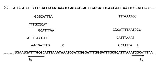
Figure 1: Process of boundary management.
Elimination of reads
Now our interest is on those reads ri, which are supposed to be aligned or mapped to the locus from x-δx to y+δy (extended target region). We have aligned all the reads to the aforesaid region. We have considered at most 2 bp difference for mapping a read ri to an extended target region; otherwise, read ri is said to be unmapped to the target locus. We have aligned the reads to the extended target boundary and measured the score with a simple point to point similarity match score [7].
Example: In Figure 2, we have shown that the reads ATTTAAATA, GGATTTGG, AATC- GATCG and TTGCGCATT are mapped to the target region. The reads GAAG-GATTT and CGCATTTAA are unmapped to the target region, which is marked by ‘x’. Now we shall consider only those reads which are mapped in x-δx to y+δy.
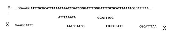
Figure 2: Process of elimination of reads.
Reconstruction of the target sequence using Ant-Target Algorithm
Our methodology Ant-Target Algorithm is based on the notion of Ant Colony Optimization algorithm. Ant colony optimization (ACO) is a population-based metaheuristic methodology, which is used to generate solutions of hard combinatorial optimization problems. In ACO, each individual in the population is an artificial agent (ant). An ant creates gradually and probabilistically a solution for a given problem. Ants build solutions by moving on a graph-based representation of the given problem. At each step, the ant adds a solution component to the partial solution. Here component means any unvisited vertex (place) of the graph. A probabilistic model is associated with the graph, which is used to motivate ants’ choices. The probabilistic model is updated dynamically by the ants, which will increase the probability to generate a good solution to be generated by future ants [8].
Now we shall define the following terms that are used in the ACO algorithm for our problem.
Graph: A graph (G) is constructed, where each vertex is a read. Here reads are actually those m reads which are mapped to the target genome. Weight of the edge/arc between ith and jth vertices is wij, depicting the extent of overlap between ith and jth reads.
Vertex/Node: Each vertex/node of a graph is basically mapped to a place, which depicts a read.
Ant: Each ant will be mapped to an artificial agent in the program. Pheromone: Pheromone (τ) is global information about the distance (Inverse distance) from a location to a food source. Here distance is mapped to the alignment score. Pheromone (τij) is updated to each arc connecting ith and jth vertices.
Local heuristics (local bias): Local heuristics (W=(wij)) is used to describe the local bias and is mapped to the overlap between the reads. Let m be the number of reads that are mapped to the target genome sequence in S. Each element wij of W is the number of bases that are similar in the direction of tail end of ith read and head end of jth read. The objective is to reconstruct the target region by assembling some of these reads. Each read is now considered as a place. Let us consider τ0=(τ01, ...τ0j, ...τ0m)T as pheromone intensity vector, such that τ0j (j=1, 2, 3,…m) quantifies the pheromone intensity from the dummy place to jth place. Let us consider the pheromone intensity matrix as T=[τij]m × m, where τij denotes the pheromone trail intensity on the path or arc from ith position (place) to jth position (place) (Figure 3). Initially some random values have been assigned to τij, say in [1, 50]. Since the starting read is unknown to us for given target region, we have to consider a dummy starting place [9].
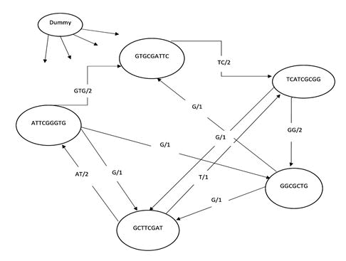
Figure 3: Equivalent graph with possible movements using the matrix W.
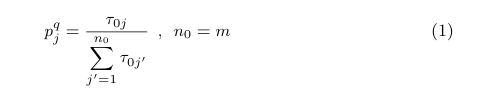
Assume that m ants are considered to be gathered at the dummy starting location. They are ready to move from the dummy place to the other unvisited places, which is based on certain probability. A qth ant will move from the dummy place to jth place based on the probability value, which is given by
Assume that one of the ants has moved to ith place or presently at ith place. Now the probability that qth ant will travel from ith place to jth place,
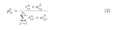
The term ni is the number of adjacent places to ith place, which still remain unvisited. In equation 2, if α=0, then the probability of movement from ith place to jth place is proportional to wβij, which is actually the case of greedy algorithm. On the other hand, if β=0, then only pheromone intensity is at work. We have observed the effect of different values of α and β and realized that the results are favorable when α and β values are 1 and 3 respectively.
Now, we have to find out the solution for the target region. In other words, we have to find an optimal path from the dummy starting place to a place where the length (l) of the partial solution is greater than θ, θ being the threshold value of l depicting the length of the extended target genome sequence. A partial solution is an intermediate sequence that will be obtained during the movement of ants. An ant can move from one place to another place using equation (1) or (2).
Example: An ant can start a journey from the dummy node and travel to the next place ATTCGGGTG (using equation (1)). After the first move, the partial solution can be ATTCGGGTG. Now from the present place ATTCGGGTG, if the ant goes to GTGCGATTC (using equation (2)), then the partial solution can be GTGCGATTCCGATTC. The reads ATTCGGGTG and GTGCGATTC have 3bp of overlapping. Assume that the ant goes from the present place GTGCGATTC to the following place TCATCGCGG (using equation (2)). Then the partial solution will be GTGCGATTCCGATTCATCGCGG. Here the reads GTGCGATTC and TCATCGCGG have a 2bp of overlapping. In this way, the partial solution length will increase, and eventually, it will cross the threshold value θ. Here θ is the difference between the extended boundaries of x and y.
In this way, a qth ant will finish the tour and the alignment score of the resulting reassembled sequence Sθ with the target region (effective target region) is measured. We have measured the alignment score using a simple point-to-point similarity match score. Before alignment, we must reset Sθ’s location with the extended boundary. Let us assume that start is effectively an extended boundary on the left side. Then after the completion of each tour, we must extract the substring from Sθ, starting from x-start to y-start, where x and y are the left and right boundaries. Let us assume that SCq is a score that corresponds to qth ant (Score of assembled Targeted region with respect to the original one). Now the ants will go back to the dummy place through an identical path (Reverse path). During the backward movement, they deposit pheromones. Pheromones are deposited on the arc (only to the path that has been traveled by an ant). Pheromone modification for τij value, is done when a qth ant goes from ith place to jth place during its way back. The value of τij is modified by

where Δτqij the pheromone amount dropped by qth ant on the arc joining ith and jth locations or places. Here Pq (arcs on the path of qth ant) is the path of qth ant. We can write the termΔτqij as Δτqij ij=SCq, where qth ant has completed a tour along Pq. Otherwise, it is zero.
There will be uniform pheromone decay on all the arcs between pairs of places. Now we can write for the arcs connecting ith and jth places as

The value of ρ lies in [0, 1) and is called the pheromone decay rate. The pheromone decay process is used to avoid uncontrolled pheromone deposits which may lead to forget the bad decisions also. After the evaporation (decay) process is over, the ants will deposit their pheromone on the arcs that they have traveled in their tour. The corresponding pheromone detail is updated by equation (4). The ants will move in parallel from the dummy place to the other places. Here the number of ants that move in parallel in each iteration is equal to the number of mapped reads. This process will continue for a finite number of iterations to get an optimal solution. After every tour of ants, we must ensure to save the best tour of the ants. Here tour refers to a solution and the best tour is indicated by the substring of Sθ (xstart to y-start) with the best alignment score.
Calculation of error
After completion of the tour, we calculate the extent by which the solution is perfect. The percentage of error is calculated by the following equation

where final score is best score of targeted assembled seq w.r.t actual sequence.
Implementation issue
We have obtained the data sequence from NCBI and Ensembl BioMart. An original DNA sequence has been mutated to form a new sequence so that it becomes 99% similar to the original one. Now we have the new sequence which is considered as an unknown sequence and it has been split further into long reads. The known original DNA sequence is now considered as the reference sequence. Now we have created long reads with length between 500 bp and 1000 bp with 5X coverage. We have deleted a few reads randomly. This is done to simulate the fact that some reads may be lost during biochemical process. Normalization of pheromone intensity values (τij and τj) are required after every iteration, otherwise, there will be an overflow. One iteration comprises m forward movement and m backward movement. The pheromone values are in [1, 50]. The value of SCq is always considered positive. After reassembling the reads, if the alignment score is negative, the score is considered as zero. The Roulette wheel concept is used to determine the probability of selection of the next place (using equation (1) and (2)). For the first iteration, ith ant is forced to jump first to ith place. This bias is given for the complete exploration of all places.
Results and Discussion
In this section, we explain the effectiveness of Ant-Target Algorithm (ATA) for genome target sequencing. The novelty of ATA over some state-of-the-art results has been established.
Data sets
Here, we have considered 20 different sequences from Ensembl BioMart and NCBI, in the organisms, like coronavirus, human, mouse, cat, zebrafish, dog, chimpanzee, lion, tiger, monkey, tortoise, camel, chicken, goat, duck, crow, budgerigar bird, atlantic salmon fish, blue whale and catfish (Table 2). We have considered all these sequences in FASTA format. All these original sequences have been considered as reference sequences.
Table 2 shows the sources and sizes of the sequences.
| Sequence | Species | Source | Length (bp) |
| 1 | Severe acute respiratory syndrome coronavirus 2 isolate Wuhan-Hu-1, complete genome | NCBI | 29902 |
| 2 | Homo_sapiens.GRCh38.dna.chromosome.1- Human | BioMart | 248956421 |
| 3 | Mus_musculus.GRCm39.dna.chromosome.1- Mouse | BioMart | 195154278 |
| 4 | Felis_catus.Felis_catus_9.0.dna.chromosome.Al-Cat | Biomart | 242100912 |
| 5 | Danio_rerio.GRCz11.dna.chromosome.1- Zebrafish | BioMart | 59578281 |
| 6 | Canis_lupus_familiaris.ROS_Cfam_1.0.dna.primary_assembly.1-DOG | BioMart | 123313938 |
| 7 | Pan_troglodytes.Pan_tro_3.0.dna.chromosome.10-Chimpanzee | BioMart | 135926726 |
| 8 | Panthera_leo.PanLeo1.0.dna.primary_assembly. A1-Lion | BioMart | 150556862 |
| 9 | CM043898.1 Panthera tigris isolate Kylo-ren chromosome A1, whole genome shotgun sequence-Tiger | NCBI | 234482688 |
| 10 | Saimiri boliviensis boliviensis isolate 100643 breed Bolivian squirrel monkey unplaced genomic scaffold Super-Scaffold_100001, whole genome shotgun sequence-Monkey | NCBI | 151810503 |
| 11 | Gopherus_evgoodei.rGopEvg1_v1.p.dna.primary_assembly. 10 (Goodes Thornscrub Tortoise) | BioMart | 86493506 |
| 12 | Camelus_dromedarius. Cam Dro2.dna.primary assembly.1 (Arabian Camel) | BioMart | 124992372 |
| 13 | Gallus_gallus.bGalGall.mat.broiler.GRCg7b.dna.primary_assembly.1 (Chicken) | BioMart | 196449155 |
| 14 | Capra_hircus.ARS1.dna.chromosome.1 (Goat) | BioMart | 157403527 |
| 15 | Anas_platyrhynchos_platyrhynchos.CAU_duck1.0.dna.primary_assembly.1 (Duck) | BioMart | 202396092 |
| 16 | Corvus_moneduloides.bCorMon1.pri.dna.primary_assembly.1 (New Caledonian Crow) | BioMart | 165740462 |
| 17 | Melopsittacus_undulatus.bMelUnd1.mat.Z.dna.primary_assembly.1 (Budgerigar bird) | BioMart | 155071705 |
| 18 | Salmo_salar Ssal_v3.1.dna.primary_assembly.1 (Atlantic Salmon fish) | BioMart | 174498728 |
| 19 | Balaenoptera_musculus.mBalMus1.v2.dna.primary_assembly.1 (Blue Whale) | BioMart | 185157307 |
| 20 | Ictalurus_punctatus.IpCoco_1.2.dna.primary_assembly.1 (Channel Catfish) | BioMart | 37510254 |
Table 2: Data sets.
Performance
Here in this section we have compared the results obtained by the proposed algorithm with the latest modern methodologies.
• A hybrid algorithm has been developed using the ReFHap algorithm and DGS algorithm. It uses the long reads of PacBio HiFi and Nanopore sequencing. They have achieved the highest accuracy in the form of genome fraction 99.971%. Genome fraction is the total number of aligned bases in the reference, divided by the genome size.
• GlodRush algorithm is a linear time complexity long reads assembly algorithm (Overlap-Layout-Consensus). It is a hybrid form of GoldPath, GoldPolish, Tigmint-long, and GoldChain. It used nanopore sequencing reads. The algorithm had achieved 99% base accuracy.
• A assembly algorithm inspector has been developed, which used long reads of PacBio CLR, PacBio HiFi and Oxford nanopore. The developer has used five standard assemblers Canu, Flye, wtdbg2, hifiasm and Shasta. They have achieved a maximum of 99.38% Mapping Ratio (MR).
• A hybrid assembly algorithm has been developed using IonTorrent and MinION reads. This algorithm uses the short reads of IonTorrent and the long reads of MinIon. The developer used some assemblers like AssemblerSPAdes, Minimap+Miniasm+Racon (Hybrid assembler), Canu+unicycler (Hybrid assembler) and Canu +unicycler+pilonX3 (Hybrid assembler). They have achieved 99.95% of ANI accuracy (maximum). ANI is Average Nucleotide Identity.
The proposed methodology ATA has reached 100% accuracy in most of the cases which we have elaborated (result) in Table 3. In column 1 of Table 3, we have shown the sequence number. Corresponding sequence details are provided in Table 2. Column 2 of Table 3 gives the average number of reads created from the given sequence. Column 3 provides the actual number of average reads mapped to the targeted region. Column 4 defines the average time (sec) required for the extended boundary calculation. The average elimination time (sec) is designated in column 5. Average Matrix creation time (sec) and assembling time (sec) are mentioned in columns 6 and 7. The average assembling error per sample is mentioned in column 8. Assembling error is calculated in terms of percentage using equation 5. For example, for row number 1 of Table 3, where we have collected the sequence “Severe acute respiratory syndrome coronavirus 2 isolate Wuhan-Hu-1, complete genome”, the total number of reads generated is 161 (column 2 of Table 3). Among these 161 reads only 56 reads are mapped to the target location (extended target location). Time required for boundary management (extended boundary) is 7 seconds. 28 seconds is required to eliminate the unnecessary reads. The matrix creation time is almost zero which can’t be tracked in terms of seconds. The Assembling time or reconstruction time of the target region is 417 seconds. The average assembling error per sample is 0.0%. Here we have taken random target regions with target size 10000bp and finally averaged the error. In another example, if we see row 20 there we will get the sequence “Ictalurus punctatus.IpCoco 1.2.dna.primary assembly.1”. The total number of reads created during the process of read creation is 197497. Only 58 reads are mapped to the extended target regions. 2579 seconds is taken for Boundary management. The elimination time for this instance is 14609 seconds. Matrix creation time is here NIL. The Assembling time is only 428 seconds. The average assembling error per sample is 0.0%. If we observe the data sequence 3, we get error percentages of 0.1%. For the remaining sequences, we got always zero errors. It means 100% accuracy. As a result, we can say that 95% time we got 100% accuracy for target sequencing. Matrix creation time is much less, which depends on the number of mapped reads. Almost every time we got zero seconds for matrix creation time. In the case of row no, 3 only we get the results in seconds, which is due to the high number of mapped reads.
| Seq # | Total reads | Mapped reads | Boundary management time | Elimination time | Matrix creation time | Assembling time | Percentage of assembling error |
| 1 | 161 | 56 | 7 | 28 | 0 | 417 | 0 |
| 2 | 1311038 | 65 | 17134 | 90585 | 0 | 484 | 0 |
| 3 | 1027659 | 564 | 13435 | 78162 | 53 | 4224 | 0.1 |
| 4 | 1274878 | 59 | 16632 | 93562 | 0 | 440 | 0 |
| 5 | 313877 | 58 | 4100 | 22297 | 0 | 430 | 0 |
| 6 | 649517 | 54 | 8485 | 43663 | 0 | 398 | 0 |
| 7 | 716013 | 60 | 9347 | 52540 | 0 | 443 | 0 |
| 8 | 792634 | 58 | 10364 | 55709 | 0 | 431 | 0 |
| 9 | 1234613 | 56 | 16188 | 88032 | 0 | 415 | 0 |
| 10 | 799490 | 60 | 10455 | 57153 | 0 | 448 | 0 |
| 11 | 455494 | 57 | 5973 | 32905 | 0 | 425 | 0 |
| 12 | 658086 | 60 | 8596 | 47961 | 0 | 447 | 0 |
| 13 | 1034398 | 56 | 13528 | 73304 | 0 | 414 | 0 |
| 14 | 828704 | 55 | 10841 | 56131 | 0 | 410 | 0 |
| 15 | 1065842 | 61 | 13923 | 76125 | 0 | 455 | 0 |
| 16 | 872893 | 57 | 11363 | 62414 | 0 | 421 | 0 |
| 17 | 816783 | 58 | 10651 | 58341 | 0 | 432 | 0 |
| 18 | 919017 | 60 | 12003 | 66727 | 0 | 445 | 0 |
| 19 | 975263 | 57 | 12684 | 71636 | 0 | 425 | 0 |
| 20 | 197497 | 58 | 2579 | 14609 | 0 | 428 | 0 |
Table 3: Result sets.
Time complexity
In this section, we have explained the overall time complexity of different methods like boundary management, elimination, matrix creation and target assembling. Let us start with the boundary management process. This boundary management function or process depends on the factor total read count and read length. Suppose Rc is the total read count and the average read length is R then according to our methodology time complexity of boundary management will be O(Rc × R2). In Figure 4 (T1 sub-figure), we have plotted the number of reads vs. time for the boundary management. The curve clearly shows it is a polynomial bounded curve.
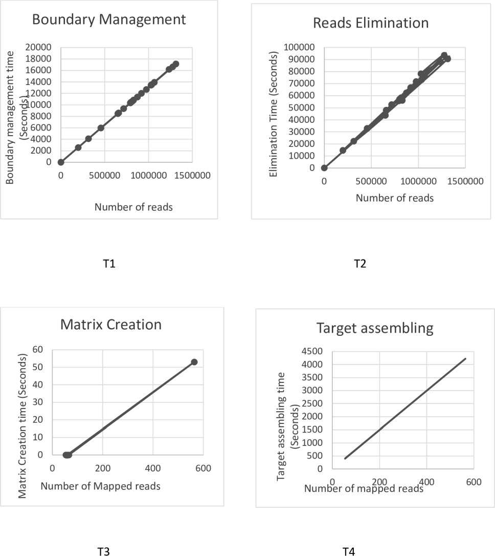
Figure 4: Time complexity for different process.
Our next point of concern is the elimination process. Which is the factor of total read count Rc, Target region size θ and average read size R. We have calculated the time complexity is about O(RC × θ × R) for the elimination process. In Figure 4 (T2 sub-figure), we have plotted the time against the number of reads. This shows that the process of elimination is polynomial-bounded. The process of matrix creation is a very less complex process. It depends on the factor number of mapped reads. If the number of mapped reads to the target region (extended target) is m then the time complexity will be O(m2). In Figure 4 (T3 sub-figure) we have plotted time against the number of mapped reads, where the curve shows the process is strictly polynomial-bounded.
The last module is target assembling which has a factor of the total number of mapped reads m. For every iteration, we have sent m number of ants. Each ant moves from one read to another read and eventually stops the tour when the partial solution length crosses threshold value θ, where θ is the difference between the extended boundary of x and y. The equation 1 and 2 has the time complexity O(m). So now the forward movement has the time complexity O(m2 × θ). The backward movement has the time complexity for m ants is O(m × θ). After completion of all tours (m tours), there is a normalization process. The normalization process has the time complexity O(m2). Hence the sequencing time complexity is Max(O(m2),O(m2 × θ),O(m × θ)). In Figure 4 we have shown the time against different numbers of mapped reads with fixed target size.Figure 4 (T4 sub-figure) depicts that sequencing time is polynomially bounded.
Conclusion
In this section, we have developed a novel Ant-Target Algorithm (ATA) for targeted DNA assembling based on Ant Colony Optimization. Target sequencing is now a very important issue, rather than whole genome sequencing. It reduces the time and data complexity. The target panels are very expensive, whereas we have developed ATA without any targeted sequencing package cost. This work needs only to clone the unknown sequence up to 5X and long reads. Once we get the reads, ATA extends the target boundary and eliminates the unnecessary reads. As a result, we get the reads which are mapped to the targeted region. The existing platforms reported >0.1% average error, whereas ATA has resulted in 0.1% maximum average error per sample. ATA has obtained 100% accuracy in 95% of the cases, which is very encouraging. The only demerit of ATA we have found that the target region we could consider is 104 bp, whereas the existing technology reaches the target region 103 bp to 107 bp. The time complexity of ATA is polynomial in nature.
Conflict of Interest
We have no conflicts of interest to disclose. All authors declare that they have no conflicts of interest.
Data Availability
There is no novel data available.
References
- Bewicke-Copley F, Kumar EA, Palladino G, Korfi K, Wang J (2019) Applications and analysis of targeted genomic sequencing in cancer studies. Comput Struct Biotechnol J 17: 1348-1359.
[Crossref] [Google Scholar] [PubMed]
- Dilliott AA, Farhan SM, Ghani M, Sato C, Liang E, et al. (2018) Targeted next-generation sequencing and bioinformatics pipeline to evaluate genetic determinants of constitutional disease. J Vis Exp 4: 57266.
[Crossref] [Google Scholar] [PubMed]
- Petrackova A, Vasinek M, Sedlarikova L, Dyskova T, Schneiderova P, et al. (2019) Standardization of sequencing coverage depth in NGS: Recommendation for detection of clonal and subclonal mutations in cancer diagnostics. Front Oncol 9: 851.
[Crossref] [Google Scholar] [PubMed]
- No JS, Kim WK, Cho S, Lee SH, Kim JA, et al. (2019) Comparison of targeted next-generation sequencing for whole-genome sequencing of Hantaan orthohantavirus in Apodemus agrarius lung tissues. Sci Rep 9: 16631.
[Crossref] [Google Scholar] [PubMed]
- Han R, Wang S, Gao X (2020) Novel algorithms for efficient subsequence searching and mapping in nanopore raw signals towards targeted sequencing. Bioinformatics 36: 1333-1343.
[Crossref] [Google Scholar] [PubMed]
- Martinez P, McGranahan N, Birkbak NJ, Gerlinger M, Swanton C (2013) Computational optimisation of targeted DNA sequencing for cancer detection. Sci Rep 3: 3309.
[Crossref] [Google Scholar] [PubMed]
- So AP, Vilborg A, Bouhlal Y, Koehler RT, Grimes SM, et al. (2018) A robust targeted sequencing approach for low input and variable quality DNA from clinical samples. NPJ Genom Med 3: 2.
[Crossref] [Google Scholar] [PubMed]
- Lo Y, Kang HM, Nelson MR, Othman MI, Chissoe SL, et al. (2015) Comparing variant calling algorithms for target-exon sequencing in a large sample. BMC Bioinformatics 16: 75.
[Crossref] [Google Scholar] [PubMed]
- Pereira R, Oliveira J, Sousa M (2020) Bioinformatics and computational tools for next-generation sequencing analysis in clinical genetics. J Clin Med 9: 132.
[Crossref] [Google Scholar] [PubMed]