Spanish
  Chinese
  Russian
  German
  French
  Japanese
  Portuguese
  Hindi
Hindi Research Article, J Chem Appl Chem Eng Vol: 1 Issue: 2
Dynamic Buffer Capacities in Redox Systems
Anna Maria MichaÅ‚owska-Kaczmarczyk1, Aneta Spórna- Kucab2 and Tadeusz MichaÅ‚owski2*
1Department of Oncology, The University Hospital in Cracow, 31-501 Cracow,
Poland
2Department of Analytical Chemistry, Technical University of Cracow, 31-155
Cracow, Poland
*Corresponding Author : Tadeusz Michałowski
Faculty of Chemical Engineering and Technology, Cracow University of Technology, Warszawska 24, 31-155 Cracow, Poland
Tel: +48126282035
E-mail: michalot@o2.pl
Received: October 04, 2017 Accepted: October 19, 2017 Published: October 24, 2017
Citation: MichaÅ‚owska-Kaczmarczyk AM, Spórna-Kucab A, MichaÅ‚owski T (2017) Dynamic Buffer Capacities in Redox Systems . J Chem Appl Chem Eng 1:2 doi:10.4172/2576-3954.1000107
Abstract
The buffer capacity concept is extended on dynamic redox systems, realized according to titrimetric mode, where changes in pH are accompanied by changes in potential E values; it is the basic novelty of this paper. Two examples of monotonic course of the related curves of potential E vs. Φ and pH vs. Φ relationships were considered. The systems were modeled according to GATES/GEB principles.
Keywords: Thermodynamics of electrolytic redox systems; Buffer capacity; GATES/GEB
Introduction
The buffer capacity concept is usually referred to as a measure of resistance of a solution (D) on pH change, affected by an acid or base, added as a titrant T, i.e., according to titrimetric mode; in this case, D is termed as titrand.
The titration is a dynamic procedure, where V mL of titrant T, containing a reagent B (C mol/L), is added into V0 mL of titrand D, containing a substance A (C0 mol/L). The advance of a titration B(C,V) ⟹ A(C0,V0), denoted for brevity as B ⟹ A, is characterized by the fraction titrated [1-4]
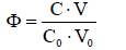 (1)
(1)
that introduces a kind of normalization (independence on V0 value) for titration curves, expressed by pH = pH(Φ), and E = E(Φ) for potential E [V] expressed in SHE scale. The redox systems with one, two or more electron-active elements are modeled according to principles of Generalized Approach to Electrolytic Systems with Generalized Electron Balance involved (GATES/GEB), described in details in [5-16], and in references to other authors’ papers cited therein.
According to earlier conviction expressed by Gran [17], all titration curves: pH = pH(Φ) and E = E(Φ), were perceived as monotonic; that generalizing statement is not true [7], however. According to contemporary knowledge, full diversity in this regard is stated, namely: (1°) monotonic pH = pH(Φ) and monotonic E = E(Φ) [18-20]; (2°) monotonic pH = pH(Φ) and non-monotonic E = E(Φ) [6]; (3°) non-monotonic pH = pH(Φ) and monotonic E = E(Φ) [5]; (4°) non-monotonic pH = pH(Φ), and nonmonotonic E = E(Φ) [7].
Examples of titration curves pH = pH(Φ) and E = E(Φ) in redox systems
In this paper, we refer to the disproportionating systems: (S1) NaOH ⟹ HIO and (S2) HCl ⟹ NaIO, characterized by monotonic changes of pH and E values during the related titrations (i.e., the case 1°). In both instances, the values: V0=100, C0=0.01, and C=0.1 were assumed. The set of equilibrium data [18-20] applied in calculations, presented in Table 1, is completed by the solubility of solid iodine, I2(s), in water, equal 1.33∙10-3 mol/L. The related algorithms, prepared in MATLAB for S1 (NaOH ⟹ HIO) S2 (HCl ⟹ NaIO) system according to the GATES/GEB principles, are presented in Appendices 1 and 2.
| No. | Reaction | Equilibrium equation | Equilibrium data |
|---|---|---|---|
| 1 | I2 + 2e–1 = 2I–1 (for dissolved I2) | [I–1]2 = Ke1·[I2][e–1]2 | E01 = 0.621 V |
| 2 | I3–1 + 2e–1 = 3I–1 | [I–1]3 = Ke2·[I3–1][e–1]2 | E02 = 0.545 V |
| 3 | IO–1 + H2O + 2e–1 = I–1 + 2OH–1 | [I–1][OH–1]2 = Ke3·[IO–1][e–1]2 | E03 = 0.49 V |
| 4 | IO3–1 + 6H+1 + 6e–1 = I–1 + 3H2O | [I–1] = Ke4·[IO3–1][H+1]6[e–1]6 | E04 = 1.08 V |
| 5 | H5IO6 + 7H+1 + 8e–1 = I–1 + 6H2O | [I–1] = Ke5·[H5IO6][H+1]7[e–1]8 | E05 = 1.24 V |
| 6 | H3IO6–2 + 3H2O + 8e–1 = I–1 + 9OH–1 | [I–1][OH–1]9 = Ke6·[H3IO6–2][e–1]8 | E06 = 0.37 V |
| 7 | HIO = H+1 + IO–1 | [H+1][IO–1] = K11I·[HIO] | pK11I = 10.6 |
| 8 | HIO3 = H+1 + IO3–1 | [H+1][IO3–1] = K51I·[HIO3] | pK51I = 0.79 |
| 9 | H4IO6–1 = H+1 + H3IO6–2 | [H+1][H3IO6–2] = K72·[H4IO6–1] | pK72 = 3.3 |
| 10 | Cl2 + 2e–1 = 2Cl–1 | [Cl–1]2 = Ke7·[Cl2][e–1]2 | E07 = 1.359 V |
| 11 | ClO–1 + H2O + 2e–1 = Cl–1 + 2OH–1 | [Cl–1][OH–1]2= Ke8·[ClO–1][e–1]2 | E08 = 0.88 V |
| 12 | ClO2–1 + 2H2O + 4e–1 = Cl–1 + 4OH–1 | [Cl–1][OH–1]4 = Ke9·[ClO2–1][e–1]4 | E09 = 0.77 V |
| 13 | HClO = H+1+ ClO–1 | [H+1][ClO–1] = K11Cl·[HClO] | pK11Cl = 7.3 |
| 14 | HClO2 + 3H+1 + 4e–1 = Cl–1 + 2H2O | [Cl–1] = Ke10·[HClO2][H+1]3[e–1]4 | E010 = 1.56 V |
| 15 | ClO2 + 4H+1 + 5e–1 = Cl–1 + 4H2O | [Cl–1] = Ke11·[ClO2][H+1]4[e–1]5 | E011 = 1.50 V |
| 16 | ClO3–1 + 6H+1 + 6e–1 = Cl–1 + 3H2O | [Cl–1] = Ke12·[ClO3–1][H+1]6[e–1]6 | E012 = 1.45 V |
| 17 | ClO4–1 + 8H+1 + 8e–1 = Cl–1 + 4H2O | [Cl–1] = Ke13·[ClO4–1][H+1]8[e–1]8 | E013 = 1.38 V |
| 18 | 2ICl + 2e–1 = I2 + 2Cl–1 | [I2][Cl–1]2= Ke14·[ICl]2[e–1]2 | E014 = 1.105 V |
| 19 | I2Cl–1 = I2 + Cl–1 | [I2][Cl–1] = K1·[I2Cl–1] | logK1 = 0.2 |
| 20 | ICl2–1 = ICl + Cl–1 | [ICl][Cl–1] = K2·[ICl2–1] | logK2 = 2.2 |
| 21 | H2O = H+1 + OH-1 | [H+1][OH-1] = KW | pKW = 14.0 |
Table 1: Physicochemical data related to the systems S1 and S2
The titration curves: pH = pH(Φ) and E = E(Φ) presented in Figure 1 and Figure 2 are the basis to formulation of dynamic buffer capacities in the systems S1 and S2.

Figure 1: (A) pH = pH(Φ) and (B) E = E(Φ) relationships plotted for the system NaOH ⟹ HIO.

Figure 2: (A) pH = pH(Φ) and (B) E = E(Φ) relationships plotted for the system HCl ⟹ NaIO.
Dynamic acid-base buffer capacities βV and BV
Dynamic buffer capacity was referred previously only to acid-base equilibria in non-redox systems [3,21-23]. However, the dynamic (βV) and windowed (BV) buffer capacities can be also related to acid-base equilibria in redox systems. The βV is formulated as follows [3,21]
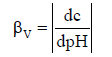 (2)
(2)
where
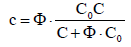
 (3)
(3)
is the current concentration of B in D+T mixture, at any point of the titration. In the simplest case, D is a solution of one substance A (C0 mol/L), and then equation 3 can be rewritten as follows
 (4)
(4)
where Φ is the fraction titrated (equation 1). Then we get
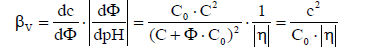 (5)
(5)
where
 (6)
(6)
is the sharpness index on the titration curve. For comparative purposes, the absolute values,|βV| and |η|, for βV (equations 1,5) and η (equation 6) are considered. At C0/C << 1 and small Φ value, from equation 3 we get
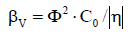
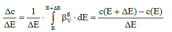
The βV value is the point–assessment and then cannot be used in the case of finite pH–changes (ΔpH) corresponding to an addition of a finite volume of titrant (βV is a non–linear function of pH). For this purpose, the ‘windowed’ buffer capacity, BV, defined by the formula [3,21]
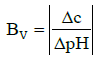 (7)
(7)
where
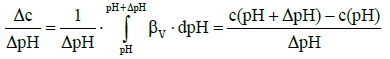 (8)
(8)
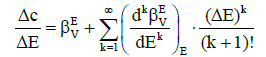
has been suggested. From extension in Taylor series we have

where
 (10)
(10)
From equations 7 and 9 we see that βV is the first approximation of BV. One should take here into account that finite changes (ΔpH) in pH, e.g. ΔpH = 1, are involved with addition of a finite volume of a reagent endowed with acid–base properties, here: base NaOH, of a finite concentration, C.
Dynamic redox buffer capacities  and
and 
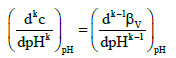
In similar manner, one can formulate dynamic buffer capacities βEV and βEV, involved with infinitesimal and finite changes of potential E values:
 (11)
(11)
 (12)
(12)
where c is defined by equation 2, and then we have
 (13)
(13)
where
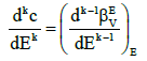 (14)
(14)
Graphical presentation of dynamic buffer capacities in redox systems
Referring to dynamic redox systems represented by titration curves presented in Figures 1,2, we plot the relationships: βV vs. Φ, βV vs. pH, βV vs. E, and βEV vs. Φ, βEV vs. pH, βEV vs. E for the systems: (S1) NaOH ⟹ HIO; (S2) HCl ⟹ NaIO. The relations: (A) βV vs. Φ, (B) βV vs. pH, (C) βV vs. E and (D) E V β vs. Φ, (E) βEV vs. pH, (F) βEV vs. E are plotted in Figures 3,4.

Figure 3: The relations: (A) βV vs. Φ, (B) βV vs. pH, (C) βV vs. E and (D) βEV vs. Φ, (E) βEV vs. pH, (F) βEV vs. E for (S1) NaOH ⟹ HIO.

Figure 4: The relations: (A) βV vs. Φ, (B) βV vs. pH, (C) βV vs. E and (D) βEV vs. Φ, (E) βEV vs. pH, (F) βEV vs. E for (S2) HCl ⟹ NaIO.
Discussion
Disproportionation of the solutes considered (HIO or NaIO) in D occurs directly after introducing them into pure water. The disproportionation is intensified, by greater pH changes, after addition of the respective titrants: NaOH (in S1) or HCl (in S2), and the monotonic changes of E = E(Φ) and pH = pH(Φ) occur in all instances.
All attainable equilibrium data related to these systems are included in the algorithms implemented in the MATLAB computer program (Appendices 1 and 2). In all instances, the system of equations was composed of: generalized electron balance (GEB), charge balance (ChB) and concentration balances for particular elements ≠ H,O.
In the system S1, the precipitate of solid iodine, I2(s), is formed (Figure 5). In the (relatively simple) redox system S2, we have all four basic kinds of reactions; except redox and acid-base reactions, the solid iodine (I2(s)) is precipitated and soluble complexes: I2Cl-1, ICl and ICl2-1 are formed (Figure 6A). Note that I2(s) + I-1 = I3-1 is also the complexation reaction.

Figure 5: Speciation diagram for the system (S1) NaOH ⟹ HIO.

Figure 6: Speciation diagram for the system (S2) HCl ⟹ NaIO: (A) for iodine species; (B) for oxidized forms of chlorine species
In the system S2, all oxidized forms of Cl-1 were involved, i.e. the oxidation of Cl-1 ions was thus pre-assumed. This way, full “democracy” was assumed, with no simplifications [18-20]. However, from the calculations we see that HCl acts primarily as a disproportionating, and not as reducing agent. The oxidation of Cl-1 occurred here only in an insignificant degree (Figure 6B); the main product of the oxidation was Cl2, whose concentration was on the level ca. 10-16 - 10-17 mol/L.
Final comments
The redox buffer capacity concepts: βV and βEV can be principally related to monotonic functions. This concept looks awkwardly for non-monotonic functions pH = pH(Φ) and/or E = E(Φ) specified above (2° - 4°) and exemplified in Figures 7,8,9. For comparison, in isohydric (acid-base) systems, the buffer capacity strives for infinity. In particular, it occurs in the titration HB (C,V) ⟹ HL (C0,V0), where HB is a strong monoprotic acid HB and HL is a weak monoprotic acid characterized by the dissociation constant K1 = [H+1][L-1]/[HL]; at 4KW/C2≪1, the isohydricity condition is expressed here by the MichaÅ‚owski formula  [24-26].

Figure 7: Case (2°): (A) monotonic pH = pH(V) and (B) non-monotonic E = E(V) plots on the step 3 of the process presented in [6].

Figure 8: Case (3°): (A) non-monotonic pH = pH(Φ) and (B) monotonic E = E(Φ) functions for the system KBrO3 ⟹ NaBr presented in [5].

Figure 9: Case (4°): the (A) non-monotonic pH = pH(Φ) and (B) non-monotonic E = E(Φ) functions for the system HI ⟹ KIO3 presented in [7].
The formula for the buffer capacity, suggested in [27] after [28], is not correct. Moreover, it involves formal potential value, perceived as a kind of conditional equilibrium constant idea, put in (apparent) analogy with the simplest static acid-base buffer capacity, see criticizing remarks in [29]; it is not adaptable for real redox systems.
Buffered solutions are commonly applied in different procedures involved with classical (titrimetric, gravimetric) and instrumental analyses [30-33]. There are in close relevance to isohydric solutions [24-26] and pH-static titration [4,34], and titration in binary-solvent systems [12,35]. Buffering property is usually referred to an action of an external agent (mainly: strong acid, HB, or strong base, MOH) inducing pH change, ΔpH, of the solution. Redox buffer capacity is also involved with the problem of interfacing in CE-MS analysis, and bubbles formation in reaction 2H2O = O2(g) + 4H+1 + 4e-1 at the outlet electrode in CE [36-39].
In Baicu et al. [40], a nice proposal of “slyke”, as the name for (acid-base, pH) buffer capacity unit, has been raised.
References
- Michałowski T (2010) The generalized approach to electrolytic systems: I. Physicochemical and analytical implications. Crit Rev Anal Chem 40: 2-16.
- Michałowski T, A Pietrzyk, M Ponikvar-Svet, M Rymanowski (2010) The generalized approach to electrolytic systems: II. The generalized equivalent mass (GEM) concept. Crit Rev Anal Chem 40: 17-29.
- Asuero AG, Michałowski T (2011) Comprehensive formulation of titration curves referred to complex acid-base systems and its analytical implications. Crit Rev Anal Chem 41: 151-187.
- MichaÅ‚owski T, Asuero AG, Ponikvar-Svet M, Toporek M, Pietrzyk A, et al. (2012) Liebig–Denigès Method of Cyanide Determination: A Comparative Study of Two Approaches. J Solution Chem 41: 1224-1239.
- MichaÅ‚owska-Kaczmarczyk AM, Asuero AG , Toporek M, MichaÅ‚owski T (2015) “Why not stoichiometry” versus “Stoichiometry – why not?” Part II. GATES in context with redox systems. Crit Rev Anal Chem 45: 240-268.
- MichaÅ‚owska-Kaczmarczyk AM, MichaÅ‚owski T, Toporek M, Asuero AG (2015) Why not stoichiometry” versus “Stoichiometry – why not?” Part III, Extension of GATES/GEB on complex dynamic redox systems. Crit Rev Anal Chem 45: 348-366.
- Michałowski T, Toporek M, Michałowska-Kaczmarczyk AM, Asuero AG (2013) New trends in studies on electrolytic redox systems. Electrochimica Acta 109: 519-531.
- Michałowski T, Michałowska-Kaczmarczyk AM, Toporek M (2013) Formulation of general criterion distinguishing between non-redox and redox systems. Electrochimica Acta 112: 199-211.
- Michałowska-Kaczmarczyk AM, Toporek M, Michałowski T (2015) Speciation diagrams in dynamic Iodide + Dichromate system. Electrochimica Acta 155: 217-227.
- Toporek M, Michałowska-Kaczmarczyk AM, Michałowski T (2015) Symproportionation versus disproportionation in bromine redox systems. Electrochimica Acta 171: 176-187.
- Michałowski T (2011) Application of GATES and MATLAB for resolution of equilibrium, metastable and non-equilibrium electrolytic systems, In: Applications of MATLAB in science and engineering. Michałowski T (edt) InTech, Rijeka, Croatia, 1-34.
- Michałowski T, Pilarski B, Asuero AG , Michałowska-Kaczmarczyk AM (2014) Modeling of acid-base properties in binary-solvent systems In: Handbook of solvents. George Wypych (edt), (1stedn) ChemTec Publishing, Toronto, 623-648.
- MichaÅ‚owska-Kaczmarczyk AM, Spórna-Kucab A, MichaÅ‚owski T (2017) Generalized electron balance (GEB) as the law of nature in electrolytic redox systems, In: Redox: principles and advanced applications, MA Ali Khalid (edt), InTech, Rijeka, Croatia, 10-55.
- MichaÅ‚owska-Kaczmarczyk AM, Spórna-Kucab A , MichaÅ‚owski T (2017) Principles of titrimetric analyses according to GATES, In: Advances in titration techniques Vu Dang Hoang (Edt), InTech, Rijeka, Croatia, 133-171.
- MichaÅ‚owska-Kaczmarczyk AM, Spórna-Kucab A , MichaÅ‚owski T (2017) Principles of titrimetric analyses according to GATES, In: Advances in titration techniques Vu Dang Hoang (Edt), InTech, Rijeka, Croatia, 133-171.
- MichaÅ‚owska-Kaczmarczyk AM, Spórna-Kucab A , MichaÅ‚owski T (2017) A distinguishing feature of the balance 2∙f(O) – f(H) in electrolytic systems. The reference to titrimetric methods of analysis, In: Advances in titration techniques, Vu Dang Hoang (edt), InTech, Rijeka, Croatia, 174-207.
- MichaÅ‚owska-Kaczmarczyk AM, Spórna-Kucab A , MichaÅ‚owski T (2017) Some remarks on solubility products and solubility concepts, In: Descriptive inorganic chemistry. Researches of metal compounds T Akitsu (edt), InTech, Rijeka, Croatia, 93-134.
- Gran G (1988) Equivalence volumes in potentiometric titrations. Anal Chim Acta 206: 111-123.
- Meija J, Michałowska-Kaczmarczyk AM, Michałowski T (2017) Redox titration challenge. Anal Bioanal Chem 409: 11-13.
- Michałowski T, Michałowska-Kaczmarczyk AM, Meija J (2017) Solution of redox titration challenge. Anal Bioanal Chem 409: 4113-4115.
- Toporek M, Michałowska-Kaczmarczyk AM, Michałowski T (2014) Disproportionation reactions of HIO and NaIO in static and dynamic systems. Am J Analyt Chem 5: 1046-1056.
- Michałowska-Kaczmarczyk AM, Michałowski T (2015) Dynamic buffer capacity in acid-base systems. J Solution Chem 44: 1256-1266.
- Michałowska-Kaczmarczyk AM, Michałowski T, Asuero AG (2015) Formulation of dynamic buffer capacity for phytic acid.Am J Analyt Chem 2: 5-9.
- Michałowski T, Asuero AG (2012) New approaches in modelling the carbonate alkalinity and total alkalinity. Crit Rev Anal Chem 42: 220-244.
- Michałowski T, Pilarski B, Asuero AG, Dobkowska A (2010) A new sensitive method of dissociation constants determination based on the isohydric solutions principle. Talanta 82: 1965-1973.
- Michałowski T, Pilarski B, Asuero AG, Dobkowska A, Wybraniec S (2011) Determination of dissociation parameters of weak acids in different media according to the isohydric method. Talanta 86: 447-451.
- Michałowski T, Asuero AG (2012) Formulation of the system of isohydric solutions. J Analyt Sci Methods Instrumentation 2: 1-4.
- Bard AJ, Inzelt G, Scholz F (edts) (2012) Electrochemical dictionary (2nd edtn), Springer-Verlag Berlin Heidelberg, Germany, 87.
- de Levie R (1999) Redox bufferstrength.J Chem Educ 76: 574-577.
- MichaÅ‚owska-Kaczmarczyk AM, Asuero AG, MichaÅ‚owski T (2015) “Why not stoichiometry” versus “Stoichiometry – why not?” Part I. General context. Crit Rev Anal Chem 45: 166-188.
- Michałowski T, Baterowicz A, Madej A, Kochana J (2001) Extended Gran method and its applicability for simultaneous determination of Fe(II) and Fe(III). Anal Chim Acta 442: 287-293.
- Michałowski T, Toporek M, Rymanowski M (2005) Overview on the Gran and other linearization methods applied in titrimetric analyses. Talanta 65: 1241-1253.
- Michałowski T, Kupiec K, Rymanowski M (2008) Numerical analysis of the Gran methods. A comparative study. Anal Chim Acta 606: 172-183.
- Ponikvar M, Michałowski T, Kupiec K, Wybraniec S, Rymanowski M (2008) Experimental verification of the modified Gran methods applicable to redox systems. Anal Chim Acta 628: 181-189.
- Michałowski T, Toporek M, Rymanowski M (2007) pH-Static titration: A quasistatic approach. J Chem Educ 84: 142-150.
- Pilarski B, Dobkowska A, Foks H, MichaÅ‚owski T (2010) Modelling of acid–base equilibria in binary-solvent systems: A comparative study. Talanta 80: 1073-1080.
- Smith AD, Moini M (2001) Control of electrochemical reactions at the capillary electrophoresis outlet/electrospray emitter electrode under CE/ESI-MS through the application of redox buffers. Anal Chem 73: 240-246.
- Moini M, Cao P, Bard AJ (1999) Hydroquinone as a buffer additive for suppression of bubbles formed by electrochemical oxidation of the CE buffer at the outlet electrode in capillary electrophoresis/electrospray ionization-mass spectrometry. Anal Chem 71: 1658-1661.
- Van Berkel GJ, Kertesz V (2001) Redox buffering in an electrospray ion source using a copper capillary emitter. J Mass Spectrom 36: 1125-1132.
- Shintani H (1997) Handbook of capillary electrophoresis applications. Polensky J (edt) Blackie Academic & Professional, London.