Spanish
  Chinese
  Russian
  German
  French
  Japanese
  Portuguese
  Hindi
Hindi Research Article, J Comput Eng Inf Technol Vol: 12 Issue: 6
Geometric Mean Method Combined With Ant Colony Optimization Algorithm to Solve Multi-Objective Transportation Problems in Fuzzy Environments
Ekanayake EMUSB*
Department of Physical Sciences, Rajarata University of Sri Lanka, Mihinthale, Sri Lanka
*Correspondence to: Ekanayake EMUSB, Department of Physical Sciences, Faculty of Applied Sciences, Rajarata University of Sri Lanka, Mihinthale, Sri Lanka, Tel: 94718097410; E-mail: uthpalaekana@gmail.com
Received: 25 January, 2022, JCEIT-22-52483;
Editor assigned: 28 January, 2022, Pre QC No. JCEIT-22-52483 (PQ);
Reviewed: 11 February, 2022, QC No. JCEIT-22-52483;
Revised: 25 March, 2022, Manuscript No. JCEIT-22-52483 (R);
Published: 01 April, 2022, DOI:10.4172/2324-9307.11.5.229
Citation: EMUSB E (2022) Geometric Mean Method Combined With Ant Colony Optimization Algorithm to Solve Multi-Objective Transportation Problems in Fuzzy Environments. J Comput Sci Technol 11:5.
Abstract
The Transportation Problem (TP) is a well-known subject in the field of optimization and a very prevalent challenge for businesspeople. The goal is to reduce the total transportation cost, time, and distance of delivering resources from several sources to a large number of destinations. The literature demonstrates that various approaches have been designed with a single goal in mind, although TPs are not always developed with a bi-goal in mind. Solving transportation difficulties with several objectives is a common task. In this study, a new method for addressing multi-criteria TP using geometric means, along with a novel approach of the Ant Colony Optimization algorithm (ACO) for solving multi-objective TP in a fuzzy environment. Fuzzy numbers have been used to solve real-world problems in various domains, including operations research and optimization. The ACO Algorithm has long been recognized as a viable alternative strategy for solving optimization problems. The purpose of this study is to provide a unique approach for organizing fuzzy numbers as well as enhancements to the ACO algorithm for solving the Multi-Objective TP model. Furthermore, the suggested method is quite simple, and it finds the best solution for both the balanced and unbalanced TPs. Our method, such as Geometric Mean Ant Colony Optimization Algorithm (GMACOA), outperforms other methods in terms of objective values. Numerical examples are provided to demonstrate the method in comparison to various current methods.
Keywords: Multi criteria distribution problem; Ant colony optimization algorithm; Geometric mean; Fuzzy environment
Introduction
In addition, TP is one of the most important distribution problems in Operations Research (OR). OR has numerous uses in engineering, business, and government systems. Daily, it is also employed to solve problems in the manufacturing and service industries. The TP is a well-known optimization problem in OR that takes a single objective function into account; nevertheless, in real-world applications, two or more criteria are more important than any single criterion. When delivering a homogeneous product from a source to a destination, the decision-maker takes numerous aspects into account, including transportation costs, a fixed price for an open route, product delivery time, deterioration rate of commodities, and so on. The TP treats many objective functions at the same time to accommodate the criteria [1]. Proposed the transportation problem originally, while studied it in detail in the Optimal Utilization of Transportation System [2]. On the other side, created efficient methods for discovering solutions, and Charnes, Cooper, and devised the stepping stone method. Furthermore, numerous researchers are working on this topic. In this paper, we look at various methods for solving a balanced and unbalanced transportation problem using fuzzy numbers and the ant colony algorithm [3].
Fuzzy set theory has been used in a variety of domains, including OR, management science, and control theory. In real-world scenarios, supply, demand, and unit transportation costs are all uncertain [4]. Used fuzzy programming approaches to handle multi-objective linear programming issues. Several strategies for solving transportation problems in fuzzy environments are proposed in the literature, such as the concept of fuzzy set, which was introduced by Zadeh [5]. Bellman and Zadeh [6] discussed the concept of decision-making in a fuzzy environment.
Many writers have researched fuzzy linear programming problem approaches since this pioneering work, including [4]. Who demonstrated that solutions produced by fuzzy linear programming are always efficient and among others [7,8]. A fuzzy transportation problem is one in which the decision parameters are fuzzy integers. Chanas et al. studied various TP situations with interval and fuzzy parameters. The goal of the fuzzy transportation problem is to move some products from various sources to various destinations while incurring the least amount of fuzzy transportation costs and satisfying the fuzzy supply and demand requirements.
Presented a fuzzy compromised programming strategy for MOTP [9]. By giving weights to objectives, the decision maker's preferences are taken into account. Developed a preference-based fuzzy GPA to solve a MOTP with fuzzy coefficients [10]. They explain the fuzzy goal's membership function. This method converts membership functions into membership goals. The Euclidean distance function is utilized to provide the suitable preference structure of goals [11]. Provided a review of the various techniques employed in MOTP. This document compiles all possible work on MOTP and provides an overview of several methodologies such as goal programming, fuzzy techniques, and evolutionary algorithms [12]. Pandian proposed a novel way to determine a fair MOTP solution. It is suggested in this strategy to create a sum of objectives [13]. Patel proposed a new row maxima approach to solve MOTP [14]. Afwat offered a product method to solve MOTP by utilizing a fuzzy membership function [15]. Kaur proposed a simple method for determining the best linear MOTP compromise solution [16]. Khilendra proposed the Matrix maxima approach with a Pareto optimality criterion to solve MOTP [17]. Waiel F Abd El-Wahid used fuzzy programming to find the best compromise solution to a multi-objective transportation problem [13]. Maulik Mukesh and colleagues used the solving Multi-objective Transportation Problem by row maxima method. Khilendra Singh and Sanjeev Rajan proposed the Geometric Mean Method for solving multi-objective transportation problems in fuzzy environments.
Furthermore, how ants can find the shortest paths between food sources and their colony. These ideas are based on ant behavior in the wild. This concept was created using the probabilistic technique known as finding good pathways via graphs. This is known as the Ant Colony Algorithm (ACA), and it was first presented by Marco Dorigo While traveling in this manner, the ants deposit a chemical compound known as a pheromone, which aids in communication among them [18-21]. When finding the quickest path between food sources and their nest, they look for areas with high pheromone concentrations. Because ants can detect pheromones and choose the most advantageous way. Dorigo, Maniezzo, and Colorni brought the concept of the ant system into the literature. The ant algorithm with elitist ants was proposed by Dorigo. Following that, many writers researched ACA, including the max-min ant system Stutzle and Hoos the ant algorithm with additional reinforcement and the best-worst ant system among others. Many optimization issues, including transportation challenges, have been solved using ant colony techniques.
In this research, we examine Geometric Mean Combined and numerous adaptations of the ant colony algorithm utilizing Ant Colony Algorithm to Solve Multi-Objective Transportation Problems in Fuzzy Environments to identify the optimal solution.
Materials and Methods
Preliminaries: In this section, some basic definitions of fuzzy numbers are presented. The Fuzzy set theory was first formulated by Zadeh [5]. The following definitions of the fuzzy numbers and some operations on it may be useful.
Definition: A fuzzy set is a pair (X,μA) X is a set and μA: X→[0,1]. For all x∈X, μA (X) is called the membership function of x. If μA (X)=1, we say that x is Fully Included in (X,μA), and if μA (X)=0, we say that x is Not Included in (X,μA). If there exists some x∈X such that μA (X)=1, we say that (X,μA) is Normal. Otherwise, we say that (X,μA) is Subnormal.
Definition Triangular fuzzy number: A triangular fuzzy number (TFN) A Ì?=(a1,a2,a3)is FN with membership function.
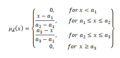
The α-cut of the TFN given by,
Aα=[a1+(a2=a1)α, a3+(a2-a3)α] (0,1). Where a1, a2 and a3 be real numbers with a1 ≤ a2 ≤ a3.
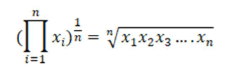
Definition geometric mean: The geometric mean is a mean or average that reveals the center tendency or typical value of a set of numbers by multiplying their values together (as opposed to the arithmetic mean which uses their sum). In general, the geometric mean is defined as the nth root of the product of n numbers, i.e., for a given set of numbers, the geometric mean is the nth root of the product of n numbers χ1, χ2,……. χn the geometric mean is defined as [22].
Mathematical model of modified ant colony algorithm (1991): Here the new path based on the probability from place i to place j for the k-th ant as shown in Equation (1).

Where, ð??ij and Ê?ij are the values of pheromone trail level of the move, and some heuristic information, which correspond to the link (i,j). ð?³ And ð?? are both parameters used to control the importance of the pheromone trail and heuristic information during component selection [23-27].
For our scenario we assumed ð??=1 and ð??=1/3 in the transition rule,
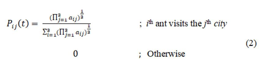
With aij; is cost between node i and node j.
Pij (t); Probability to branch from node i to node j.
Pheromone update rule.
After all ants complete their tours, the local update rule of the pheromone trails is applied for each route according to [3].
After that, apply the global pheromone update rule in which the amount of pheromone is added to the best route which has the lowest cost [28-30].
Here, Yk is the distance of the best route. µ is simply a parameter to adjust the amount of pheromone deposited, typically it would be set to 1. We sum for every solution which used component (i,j), then that value becomes the amount of pheromone to be deposited on component (i,j).
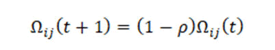
Where ð??ij (t) is the maximum number of Demands or Supplies and 0<p ≤ 1.
Mathematical formulation: The mathematical formulation of the FTP is as follows.
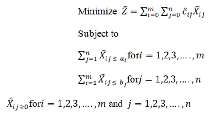
Here, all ai and bj are assumed to be positive, and ai are normally called supplies and bj are called demands, as shown in below Table. The fuzzy cost Cij is all non-negative. If ∑mi=1 ai= ∑nj=1 bj, it is a balanced transportation problem. If this condition is not met, a dummy origin or destination is generally introduced to make the problem balanced [31-32].
Proposed method: In this section, a proposed method, Improved Ant Colony Algorithm, for ï¬nding an optimal solution. Following are the steps for solving Fuzzy transportation problem.
Algorithm
Step 1: Construct the fuzzy transportation the cost table from the given problem
Step 2: Examine the TP to see if it is balanced, and if not, make it so.
Step 3: Convert fuzzy cost values in the Transportation cost table to crisp cost values by utilizing Geometric Mean.
Step 4: The probability table is then computed using the Modified ACO algorithm.
Step 5: Starting with the Xij=min(ai,bj) (unbalanced) or starting with the Xij=max(ai,bj) (balanced) probability table to make the first allocation.
Step 6: Assign, Step 5 at the place of the minimum probability cell
Step 7: If the demand in the column (or supply in the row) is satisfied, delete that column (or row), then proceed to the next minimal value in the demand and supply.
Step 8: Repeat this process until all supply and demand are satisfied, And then proceed to.
Step 9: Stop and compute the first viable solution.
Step 10: Otherwise, proceed to Step 6.
Illustration example
Example 1: We take a distribution problem in which a single homogeneous item is to be distributed from three stores (A,B,C) to four different warehouses (P,Q,R,S). Cost, time and distance for each unit transported is given in the Table. Find the minimum time, cost and distance (Table 1-11) [16].
| Supply | P | Q | R | S | Supply |
|---|---|---|---|---|---|
| Demand | |||||
| A | 21 | 16 | 15 | 13 | 11 |
| B | 17 | 18 | 24 | 23 | 13 |
| C | 32 | 27 | 18 | 41 | 19 |
| Demand | 6 | 10 | 12 | 15 | 43 |
Table 1: Cost
| Supply | P | Q | R | S | Supply |
|---|---|---|---|---|---|
| Demand | |||||
| A | 1 | 2 | 1 | 4 | 11 |
| B | 3 | 3 | 2 | 1 | 13 |
| C | 4 | 2 | 5 | 9 | 19 |
| Demand | 6 | 10 | 12 | 15 | 43 |
Table 2: Time
| Supply | P | Q | R | S | Supply |
|---|---|---|---|---|---|
| Demand | |||||
| A | 11 | 13 | 17 | 14 | 11 |
| B | 16 | 18 | 14 | 10 | 13 |
| C | 21 | 24 | 13 | 10 | 19 |
| Demand | 6 | 10 | 12 | 15 | 43 |
Table 3: Distance
| Supply | P | Q | R | S | Supply |
|---|---|---|---|---|---|
| Demand | |||||
| A | 6.13 | 7.46 | 6.34 | 8.99 | 11 |
| B | 9.34 | 9.9 | 8.75 | 6.13 | 13 |
| C | 13.9 | 10.9 | 10.53 | 15.45 | 19 |
| Demand | 6 | 10 | 12 | 15 | 43 |
Table 4: Step 3
| Supply | P | Q | R | S | Supply |
|---|---|---|---|---|---|
| Demand | |||||
| A | 0.053 | 0.065 | 0.055 | 0.078 | 11 |
| B | 0.082 | 0.086 | 0.076 | 0.053 | 13 |
| C | 0.122 | 0.095 | 0.092 | 0.135 | 19 |
| Demand | 6 | 10 | 12 | 15 | 43 |
Table 5: Step 4
| Supply | P | Q | R | S | Supply |
|---|---|---|---|---|---|
| Demand | |||||
| A | 0.053 | 0.065 | 0.055 | 0.078 | 11 |
| B | 0.082 | 0.086 | 0.076 | 0.053 | 13 |
| C | 0.122 | 0.095 | .092*12 | 0.135 | 19*7 |
| 6 | 10 | 12*0 | 15 | 43 |
Table 6: Steps 5 and 6 and 1st allocation
| Supply | P | Q | R | S | Supply |
|---|---|---|---|---|---|
| Demand | |||||
| A | 0.053 | 0.065 | 0.055 | 0.078 | 11 |
| B | 0.082 | 0.086 | 0.076 | 0.053 | 13 |
| C | 0.122 | .095*7 | .092*12 | 0.135 | 19*7*0 |
| 6 | 10*3 | 12*0 | 15 | 43 |
Table 7: Steps 6 and 7 and 2nd allocation
| Supply | P | Q | R | S | Supply |
|---|---|---|---|---|---|
| Demand | |||||
| A | 0.053 | .065*3 | 0.055 | 0.078 | 11*8 |
| B | 0.082 | 0.086 | 0.076 | 0.053 | 13 |
| C | 0.122 | .095*7 | .092*12 | 0.135 | 19*7*0 |
| 6 | 10*3*0 | 12*0 | 15 | 43 |
Table 8: Steps 6 and 7and 3rd allocation
| Supply | P | Q | R | S | Supply |
| Demand | |||||
| A | .053*6 | .065*3 | 0.055 | 0.078 | 11*8*2 |
| B | 0.082 | 0.086 | 0.076 | 0.053 | 13 |
| C | 0.122 | .095*7 | .092*12 | 0.135 | 19*7*0 |
| 6*0 | 10*3*0 | 12*0 | 15 | 43 |
Table 9: Steps 6-8 and 3rd allocation
| Supply | P | Q | R | S | Supply |
|---|---|---|---|---|---|
| Demand | |||||
| A | .053*6 | .065*3 | 0.055 | .078*2 | 11*8*2*0 |
| B | 0.082 | 0.086 | 0.076 | 0.053 | 13 |
| C | 0.122 | .095*7 | .092*12 | 0.135 | 19*7*0 |
| 6*0 | 10*3*0 | 12*0 | 15*13 | 43 |
Table 10: Steps 6-8 and 3rd allocation
| Supply | P | Q | R | S | Supply |
|---|---|---|---|---|---|
| Demand | |||||
| A | .053*6 | .065*3 | 0.055 | .078*2 | 11*8*2*0 |
| B | 0.082 | 0.086 | 0.076 | .053*13 | 13*0 |
| C | 0.122 | .095*7 | .092*12 | 0.135 | 19*7*0 |
| 6*0 | 10*3*0 | 12*0 | 15*13*0 | 43 |
Table 11: Step 9
The solution is given as: X11=6, X12=3, X13=2, X24=13, X32=7, X33=12
Following are the values of objectives: Minimum Cost=904 units, Minimum Time=107 units, Minimum distance=587 units (1 iteration) (Table 12-21).
| Method | Minimum | Minimum | Minimum |
|---|---|---|---|
| cost | time | Distance | |
| New row | 938 | 117 | 457 |
| Maxima method [9] | |||
| Product Approach | 938 | 132 | 552 |
| [10] | |||
| Geometric mean | 904 | 107 | 587 |
| method | |||
| GMACOA | 904 | 107 | 587 |
| LINGO | 796 | 89 | 527 |
Table 12: Comparison between different methods
The findings of the comparisons in Table 12 are depicted using bar graphs, as shown in Figure 1.

According to the simulation findings (Figure 1 and Table 12), the proposed strategy outperforms the geometric mean method [35].
Example 2: Now we take one more example with following characteristics [16].
| Supply |
P |
Q |
R |
S |
Supply |
|---|---|---|---|---|---|
Demand |
|||||
A |
6 |
4 |
1 |
5 |
14 |
B |
8 |
9 |
2 |
7 |
16 |
C |
4 |
3 |
6 |
2 |
5 |
Demand |
6 |
10 |
15 |
4 |
Table 13: Cost
| Supply | P | Q | R | S | Supply |
|---|---|---|---|---|---|
| Demand | |||||
| A | 13 | 11 | 15 | 20 | 14 |
| B | 17 | 14 | 12 | 13 | 16 |
| C | 18 | 18 | 15 | 12 | 5 |
| Demand | 6 | 10 | 15 | 4 |
Table 14: Time
| Supply | P | Q | R | S | Supply |
|---|---|---|---|---|---|
| Demand | |||||
| A | 6 | 3 | 5 | 4 | 14 |
| B | 5 | 9 | 2 | 7 | 16 |
| C | 5 | 7 | 8 | 6 | 5 |
| Demand | 6 | 10 | 15 | 4 |
Table 15: Distance
| Supply | P | Q | R | S | Supply |
|---|---|---|---|---|---|
| Demand | |||||
| A | 7.76 | 5.09 | 4.21 | 7.36 | 14 |
| B | 8.79 | 10.42 | 3.63 | 8.6 | 16 |
| C | 7.11 | 7.23 | 8.96 | 5.24 | 5 |
| Demand | 6 | 10 | 15 | 4 |
Table 16: Step 3
| Supply | P | Q | R | S | Supply |
|---|---|---|---|---|---|
| Demand | |||||
| A | 0.091 | 0.06 | 0.049 | 0.087 | 14 |
| B | 0.104 | 0.123 | 0.043 | 0.101 | 16 |
| C | 0.084 | 0.085 | 0.106 | 0.062 | 5 |
| Demand | 6 | 10 | 15 | 4 |
Table 17: Step 4
| Supply | P | Q | R | S | Supply |
|---|---|---|---|---|---|
| Demand | |||||
| A | 0.091 | 0.06 | 0.049 | 0.087 | 14 |
| B | 0.104 | 0.123 | .043*15 | 0.101 | 16*1 |
| C | 0.084 | 0.085 | 0.106 | 0.062 | 5 |
| Demand | 6 | 10 | 15*0 | 4 |
Table 18: Step 5 and 1st allocation
| Supply | P | Q | R | S | Supply |
|---|---|---|---|---|---|
| Demand | |||||
| A | 0.091 | .060*10 | 0.049 | 0.087 | 14*4 |
| B | 0.104 | 0.123 | .043*15 | 0.101 | 16*1 |
| C | 0.084 | 0.085 | 0.106 | 0.062 | 5 |
| Demand | 6 | 10*0 | 15*0 | 4 |
Table 19: Steps 5-7 and 1st allocation
| Supply | P | Q | R | S | Supply |
|---|---|---|---|---|---|
| Demand | |||||
| A | .091*4 | .060*10 | 0.049 | 0.087 | 14*4*0 |
| B | .104*1 | 0.123 | .043*15 | 0.101 | 16*1 |
| C | .084*1 | 0.085 | 0.106 | .062*4 | 5*1 |
| Demand | 6*5*1*0 | 10*0 | 15*0 | 4*0 |
Table 20: Steps 5-8 and other allocations
| Method | Minimum | Minimum | Minimum |
|---|---|---|---|
| cost | time | Distance | |
| New row | 122 | 461 | 130 |
| Maxima method [9] | |||
| Product Approach | 114 | 425 | 128 |
| [10] | |||
| Geometric mean | 114 | 425 | 118 |
| method | |||
| GMACOA | 114 | 425 | 118 |
| LINGO | 114 | 424 | 106 |
Table 21: Comparison between different methods
Table 21's comparison data are also depicted using bar graphs and the results Figure 2.

Figure 2: Shows a comparison of the outcomes given by the new row maxima approach, the product approach, the geometric mean method, gmacoa, and the optimal method.
The proposed technique uses the geometric mean method, according to the simulation results (Figure 2 and Table 22-28).
Example 3:
| x | D1 | D2 | D3 | Supply |
|---|---|---|---|---|
| S1 | (1,2,3) | (4,7,10) | (10,14,18) | 5 |
| S2 | (2,3,4) | (2,3.4) | (0,1,2) | 8 |
| S3 | (1,5,9) | (3,4,5) | (4,7,10) | 7 |
| S4 | (0,1,2) | (5,6,7) | (1,2,3) | 15 |
| Demand | 7 | 9 | 18 |
Table 22: Example
| x | D1 | D2 | D3 | Dummy | Supply |
|---|---|---|---|---|---|
| S1 | (1,2,3) | (4,7,10) | (10,14,18) | 0 | 5 |
| S2 | (2,3,4) | (2,3.4) | (0,1,2) | 0 | 8 |
| S3 | (1,5,9) | (3,4,5) | (4,7,10) | 0 | 7 |
| S4 | (0,1,2) | (5,6,7) | (1,2,3) | 0 | 15 |
| Demand | 7 | 9 | 18 | 1 |
Table 23: Step 2
| x | D1 | D2 | D3 | Dummy | Supply |
|---|---|---|---|---|---|
| S1 | 1.81 | 6.54 | 13.61 | 0 | 5 |
| S2 | 2.88 | 2.88 | 0 | 0 | 8 |
| S3 | 3.55 | 3.91 | 6.54 | 0 | 7 |
| S4 | 0 | 5.94 | 1.81 | 0 | 15 |
| Demand | 7 | 9 | 18 | 1 |
Table 24: Step 3
| x | D1 | D2 | D3 | Dummy | Supply |
|---|---|---|---|---|---|
| S1 | .036 | .132 | .275 | 0 | 5 |
| S2 | .058 | .058 | 0 | 0 | 8 |
| S3 | .071 | .079 | .132 | 0 | 7 |
| S4 | 0 | .120 | .036 | 0 | 15 |
| Demand | 7 | 9 | 18 | 1 |
Table 25: Step 4
| x | D1 | D2 | D3 | Dummy | Supply |
|---|---|---|---|---|---|
| S1 | .036*4 | .132 | .275 | 0*1 | 4*0 |
| S2 | .058 | .058 | 0 | 0 | 8 |
| S3 | .071 | .079 | .132 | 0 | 7 |
| S4 | 0*3 | .120 | .036*12 | 0 | 0 |
| Demand | 0 | 9 | 18 | 1 |
Table 26: Step 6 and 1st allocation
| x | D1 | D2 | D3 | Dummy | Supply |
|---|---|---|---|---|---|
| S1 | .036*4 | .132 | .275 | 0*1 | 0 |
| S2 | .058 | .058*2 | 0*6 | 0 | 0 |
| S3 | .071 | .079*7 | .132 | 0 | 7*0 |
| S4 | 0*3 | .120 | .036*12 | 0 | 0 |
| Demand | 0 | 0 | 18 | 1 |
Table 27: Other steps and other allocations
The solution is given as: X11=4, X22=2, X23=6, X32=7, X41=3, X43=12
Following are the values of objectives: 4(1,2,3)+2(2,3,4)+6(0,1,2)+7(3,4,5)+3(0,1,2)+12(1,2,3)=(41,75,109)=75
| Method | VAM | SVAM | GVAM | BVAM | RVAM | ASM | ZSM | IZPM | GMACOA | Optimal |
|---|---|---|---|---|---|---|---|---|---|---|
| Example 3 | 82 | 99 | 80 | 84 | 93 | 149 | 79 | 75 | 75 | 75 |
Table 28: Initial Solutions Obtained by all Procedures.
The comparison data from Table 24 are also represented using bar graphs and the form Figure 3.

Figure 3: A comparison of the results obtained by VAM, GVAM, BVAM, RVAM, ASM, ZSM, IZPM, GMACOA and Optimal.
According to the simulation results (Figure 3 and Table 24), the suggested strategy employs the IZPM method, and other ways outperform our GMACOA. In addition, the shortest number of iterations resulted in the best solution.
Conclusion
The TP is an essential component of this serious universe. The fundamental purpose of ordinary TPs is to reduce the cost of carrying an item from its origin to its destination. A lot of objectives must be examined and optimized concurrently in some major problems. These are known as multi-objective problems. In this work, instead of using conventional approaches, the geometric mean method combined with the Ant Colony Algorithm is used to solve a multi-objective fuzzy transportation problem in fuzzy environments. When compared to other current approaches, the proposed algorithm provides the best performance. As a result, the higher the IFS, the less iteration are required to get the final optimal solution. The method is quite straightforward. In this study, however, we provide a novel alternative method, a modified ant colony optimization algorithm that provides an optimal solution to the many different types of TPs.
Acknowledgements
This research was funded in part by an international grant from Rajarata University in Sri Lanka. Finally, I'd want to express my heartfelt gratitude to my wife, daughters, and son for their comfort and invaluable assistance at this difficult time.
Competing interests
Authors have declared that no competing interests exist.
References
- Hitchcock FL (1941) The distribution of a product from several sources to numerous localties. J Math Phys 20:224-230.
- Koopmans TC (1949) Optimum Utiliztion of Transportation System. Econometrica, United States.
- Dantzig GB (1963) Linear programming and extensions. Princeton University Press, New Jersey, United States.
- Zimmermann HJ (1978) "Fuzzy programming and linear programming with several objective functions". Fuzzy Sets Syst 1:45-55.
- Zadeh LA. (1965) " Fuzzy sets" Inf Control 8:338-353.
- Bellman RE, Zadeh LA (1970) Decision-Making in a Fuzzy Environment. Manag Sci 17:141-273.
- Fang SC, Hu CF, Wang HF, Wu SY (1999) s"Linear Programming with fuzzy coefficients in constraints". Comput Math Appl 37:63-76.
- Rommelfranger H, Wolf J, Hanuschek R (1989) Linear programming with fuzzy coefficients". Fuzzy Sets Syst 29:195-206.
- Lushu Li, Lai KK (2000) A fuzzy approach to multi-objective transportation problem. Comput Oper Res 27:43-57.
- Surapati Pramanik, Tapan k Roy (2008) Multi-objective transportation model with fuzzy parameters, Priority based fuzzy goal programming approach. J Transp Syst Eng Inf Tech 8:40-48.
- Jagtap KB, Kawale SV (2017) Multi-objective Transportation Problem with different optimization techniques: An overview. Rese gate 11:1
- Pandian P (2012) A simple approach for finding a fair solution to multiobctive programming problems. Bull Math Sci Appl 2:21-25.
- Maulik Mukesh bhai Patel, Achyut Patel C (2018)Solving multi-objective transportation problem by row maxima method. RRIJM 3.
- Afwat MAE, Salama AAM, Farouk N (2018) A new efficient approach to solve multi-objective transportation problem in the fuzzy environment (Product Approach). Int J Appl Eng Res 13:13660-13664.
- Lakhveer k, Madhuchanda R, Sandeep s (2019) A new approach to solve Multi-objective Transportation Problem. Appl Math 13:150-159.
- Khilendra Singh, Sanjeev Rajan (2020) Geometric mean method to solve multi-objective transportation problem under fuzzy environment. IJITEE 9:2278-3075
- Waiel F, Abd El-Wahed (2001) A multi objective transportation problem under fuzziness. Elsev Fuzzy sets syst 117:27-33.
- Dorigo ACM, Maniezzo V (1991)Distributed optimization by ant colonies. Proceedings of the 1st European Conference on Artificial Life 134-142.
- Dorigo M, Maniezzo V, Colorni A (1996)The ant system: Optimization by a colony of cooperating agents. IEEE Trans Syst Man Cybern B Cybern 26:29–41.
- Dorigo M, Stutzle T (2001) "An Experimental Study of the Simple Ant Colony Optimization Algorithm". WSES Inter Confe Evolu Compu 253–258.
- Dorigo M, Stutzle T, Thomas Stutzle (2004) Ant colony optimization. MIT Press, Europe.
- Krishna Prabha S (2021) Geometric mean with pythagorean fuzzy transportation problem. Turk J Comput Math Educ 12:1171-1176
- Edward Samuel A, Venkatachalapathy M (2013) Izpm for unbalances fuzzy transportation problems. Int J Pure Appl Math 86:689-700
- Amarpreet K, Amit K (2011)A new approach for solving fuzzy transportation problems using generalized trapezoidal fuzzy numbers. Appl Soft Comput 1-34:2011.
- Arsham H, Khan AB (1989) A simplex type algorithm for general transportation problems: An alternative to stepping stone. J opl res 40:581-590.
- Charnes A, Cooper WW (1970) The stepping stone method of explaining linear programming calculations in transportation problems. Manag Sci 1:49-69.
- Chen SH, Hsieh CH (1999) Graded mean integration representation of generalized fuzzy numbers. Journal of The Chinese Fuzzy Systems Association 5:1-7.
- Chen SM, Chen JH (2009) Fuzzy risk analysis based on the ranking generalized fuzzy numbers with different heights and different spreads. Expert Syst Appl 36:6833-6842.
- Dong G, Guo WW (2010) A cooperative ant colony system and genetic algorithm for TSPs. Adv Swar Intel 597-604.
- Dorigo M, DiCaro G (1999) The ant colony optimization meta-heuristic. McGraw-Hill Ltd, UK, Maidenhead, UK, England.
- Dorigo M, Caro GD, Gambardella LM (1999) Ant algorithms for discrete optimization," Artif Life 5:137–172.
- Dorigo M, Gambardella LM (1997) Ant colony system: A cooperative learning approach to the traveling. IEEE Transactions on Evolutionary Computation. ;1:53-66.
- Ekanayake EMUSB, Perera SPC, Daundasekara WB, Juman JAMS (2020) A Modified Ant Colony Optimization Algorithm for Solving a Transportation Problem. J adv math comput 35:83-101.
- Kaufmann A, Gupta MM (1991) Introduction to fuzzy arithmetics: Theory and applications. Van Nostrand Reinhold, New York.
- Shan-Huo Chen (1999) Graded mean integration representation of generalized fuzzy numbers. J Chinese Fuzzy Syst Asso 5:1-7.