Spanish
  Chinese
  Russian
  German
  French
  Japanese
  Portuguese
  Hindi
Hindi Research Article, J Appl Bioinformat Computat Biol S Vol: 10 Issue: 4
Objective Comparison of High Throughput qPCR Data Analysis Methods
Mathieu Bahin, Marine Delagrange, Quentin Viautour, Juliette Pouch, Amine Ali Chaouche, Bertrand Ducos and Auguste Genovesio*
Departement de Biologie, Institut de Biologie de l’ENS (IBENS), Ecole Normale Superieure, CNRS, INSERM, Universite PSL, 75005 Paris, France
*Corresponding Author: Auguste Genovesio
Departement de Biologie, Institut de Biologie de l’ENS (IBENS), Ecole Normale Superieure, CNRS, INSERM, Universite PSL, 75005 Paris, France
E-mail: auguste.genovesio@ens.fr, bertrand.ducos@phys.ens.fr
Received: September 28, 2021 Accepted: October 18, 2021 Published: October 25, 2021
Citation: Bahin M, Delagrange M, Viautour Q, Pouch J, Chaouche AA, et al. (2021) Objective Comparison of High Throughput qPCR Data Analysis Methods. J Appl Bioinforma Comput Biol S4.
Abstract
For the past 25 years, real time quantitative PCR (qPCR) has been the method of choice to measure gene expression in biological research and diagnosis using semi-automated data analysis methods adapted to low throughput. Recently, modern platforms have largely increased the throughput of samples and a single HTqPCR experiment can produce up to ten thousand reaction curves, requiring full automation. An extensive comparison of these methods in this new context has not yet been performed. In consequence, the community has not yet named a reference method to analyze HT-qPCR data. In this work, we aim to evaluate and compare available qPCR data analysis methods when ported to high throughput. In order to perform such comparison on a common ground, we developed a preprocessing approach based on the design of a robust high throughput fitting to correct bias and baseline prior to further quantification of gene expression by individual methods. Using four quantitative criteria, we then compared results obtained on high throughput experiments using five reference methods designed for low throughput qPCR data analysis (Cq, Cy0, logistic5p, LRE, LinReg) as well as deep learning. The advantages and disadvantages of these methods in this new context were discussed. While deep learning presents the advantage of not requiring any preprocessing steps, we nevertheless conclude that Cq, one of the oldest method, because of its simplicity, its robustness to dataset variability, and the fact that it doesn’t require a large training set, should be preferred over other approaches to analyze high throughput qPCR experiments.
Keywords: DrugReceptor Interactions, Computational Approach
Introduction
Polymerase chain reaction, designed in the mid 80’s in order to generate billions of copies from a small DNA sample, is a widely used technique with a broad set of applications in biological research and medicine [1,2]. Development of real time or quantitative polymerasechain- reaction (qPCR) followed in the next decade. This consists of monitoring the reaction in real time, thus allowing indirect access to the amplification efficiency. Consequently, qPCR significantly increased the precision of gene copy quantification [3]. For about ten years, the throughput of qPCR that could be performed in parallel has also significantly increased. It followed the rise of microfluidic devices that allow miniaturization of individual reactions at a nanoliter scale [4,5]. In practice, whatever the throughput, qPCR produces amplification curves that need to be analyzed and quantified.
To date, numerous data analysis strategies have been proposed in order to extract meaningful information from qPCR curves [3,6-9]. While absolute quantification is, in theory, an interesting goal, its usefulness is questionable in a high throughput context [10]. To our understanding, a relative comparison of gene copy between samples covers most applications [11]. These methods were notably developed in the context of low throughput qPCR experiments, where each reaction could still be visually investigated and analysis manually curated. As a consequence, they were mostly designed as semiautomated. However, going from one or a bunch of qPCR curves to thousands of them raises concrete issues since manual intervention is no longer an option. High throughput qPCR requires analysis to be both fully automated and robust. From this point, what existing data analysis methods can be ported to high throughput? What method performs best when applied to high throughput experiments?
In this work, we conducted an objective comparison of the performance of six data analysis methods (Cq, Cy0, logistic 5p, LRE, LinReg and deep learning), when applied to the same high throughput qPCR data sets designed to this end, where initial gene copy numbers were known. In order to perform a relevant comparison focusing only on the choice of the data analysis strategy for gene copy comparison, we developed a robust preprocessing pipeline that corrected raw data prior to execution of data analysis methods per se. Starting from this common ground made possible a fair comparison of the quantification methods, all other factors being equal. This preprocessing pipeline consisted firstly to sort out sigmoid curves that corresponded to actual reactions to be analyzed, from flat curves corresponding to failed reactions or empty wells, secondly, to perform the same bias and baseline corrections on them, and finally, to make both these steps robust at high throughput. We subsequently performed data analysis and reported the results obtained for each method on two plates (with respectively 568 and 894 remaining sigmoid curves) using four quantitative criteria. These criteria were all related to the final goal of such an experiment: accurately reporting an existing and repeatable difference of gene copy number between samples.
Material
Microfluidic Plates Design
Target preparation: Total RNA was extracted (RNeasy Microkit Qiagen) from fixed zebrafish (PAXgene Container Qiagen) at the 20 somite developmental stage. Quality control was conducted from 1 μL of RNA subjected capillary electrophoresis on nanoRNA chips (Bioanalyzer Agilent) and gave an RIN score equal to 9.0. The RT reaction was conducted with 1 μL of Sensiscript reverse transcriptase from 50 ng total RNA in a total volume of 20 μL, according to the supplier’s recommendations (Sensiscript RT Kit, Qiagen).
10 ng of cDNA was amplified in 20 μL final with 10 μL of 2X Gene expression Master Mix and 1 μL of each of the 16 Taqman Gene Assay (Thermofischer, Table 1) following the supplier’s protocol: 2 min at 50°C, 10 min at 95°C then 40 cycles where the samples were subjected to 95°C for 15’’ and 60°C for 60’’. The PCR products were purified with the PCR-CleanUp kit (macherey-Nagel) and re-purified in 30 μL of TE buffer. In a final volume of 6 μL, 4 μL of each PCR product was added to 1 μL of saline and 1 μL of TOPO vector and incubated for 10’ at room temperature (pCR4-TOPO cloning kit, Invitrogen). 16 aliquots of 50 μL E. coli One Shot TOP10 bacteria (Invitrogen) were transformed with 2 μL each of the cloning reactions according to the protocol: 10’ at 4°C, 30’’ at 42°C then 2’ at 4°C before being supplemented with 250 μL of SOC medium and incubated under agitation at 37°C for 1 hour. The bacteria were spread on ampicillin LB plates and incubated overnight at 37°C. After colony PCR analysis, the 16 positive clones were amplified overnight in 200 mL ampicillin LB at 37°C with agitation and the 16 plasmids were extracted and purified following the Macherey-Nagel midi prep protocol and diluted to 10 ng/μL or 50 ng/μL in low TE.
Specific target preamplification: Each standard pool was used for multiplex pre-amplification in a total volume of 5 μL containing 1 μL of 5X Fluidigm® PreAmp Master Mix, 1.25 μL of each pool standard (PS or PC), 1.25 μL of pooled TaqMan® Gene Expression assays (Life Technologies, ThermoFisher), with a final concentration of each assay (Table 1) of 180nM (0.2X) and 1.5μL of nuclease-free water. The samples were subjected to pre-amplification following the temperature protocol: 95°C for 2 min, followed by 20 cycles at 95°C for 15s and 60°C for 4 min. The pre-amplified targets were diluted 5X by adding 20 μL of low TE buffer and stored at -20°C before qPCR.
Conditions: For the considered datasets, each well corresponds to the amplification of a given gene in a sample that was diluted a given number of times. For convenience, in this manuscript, such a particular combination of gene-sample dilution is denoted “condition”. Each such condition was replicated six times.
PS samples: The targets are mixed to form standard pools (Table 2) at a rate of 5μL each at 50 ng/μL (i.e. 50/16 = 3.125 ng/μL final concentration). The standard pools are diluted 10 by 10 from PS1 to PS11, then loaded onto the plate, either directly orafter 5 preamplification runs (10, 12, 14, 16 or 18 cycles).
PC samples: The same as PS samples except that the initial target concentrations are deliberately variable (Table 2). The standard pools are diluted from PC1 to PC11 (pool concentration) then loaded onto the plate either directly or after pre-amplification.
Plate no. 1: The 16 targets were diluted to 1 ng/μL and then mixed at a rate of 5 μL each in a final 80 μL to produce standard pool 1 (PS1) representing the most concentrated mixture for each of the targets. PS1 was then diluted serially 10 by 10 to PS11. The standard pools were loaded in the 96.96 chip (IFC 96, Fluidigm), after being preamplified or not, in order to evaluate the detection limit of the targets in the plate. Each condition was replicated six times.
Plate no. 2: As in plate no. 1, the 16 targets were used to produce the 11 dilutions of the PS condition. In addition, 11 dilutions were used to produce 10 dilutions of the PC condition. Each condition for each target was replicated six times.
High Throughput qPCR: Quantitative PCR was performed using the high throughput platform BioMark™ HD System and the 96.96 GE Dynamic Arrays (Fluidigm®). The expression of 96 target genes (16 genes x 6 replicates) was quantified in 96 samples by quantitative PCR on 96.96 microfluidic chip which contained a non-template control (NTC). 6μL of Sample Master Mix (SMM) consisted of 2,7μL of each pool standard (PS or PC) or of 5X diluted pre-amplified targets, 0.3μL of 20X GE Sample Loading Reagent (Fluidigm) and 3μL of TaqMan® Gene Expression PCR Master Mix (Life Technologies, ThermoFisher). Each 6μL Master Mix Assay (MMA) consisted of 4μL of TaqMan® Gene Expression assay 20X (Life Technologies, ThermoFisher) and 4μL of 2X Assay Loading Reagent (Fluidigm). 5μL of each SMM and each MMA premixes were added to the dedicated wells. The samples and assays were mixed inside the plate using HX IFC controller (Fluidigm). The loaded Dynamic Array was transferred to the Biomark™ real-time PCR instrument and subjected to PCR experiment (25°C for 30min and 70°C for 60min for thermal mix ; 50°C for 2min and 95°C for 10min for hot start ; 40 cycles at 95°C for 15s and 60°C for 1min). The parameters of the thermocycler were set with ROX as passive reference and single probe FAM-MGB as fluorescent detector. To determine the quantification cycle Cq, data were processed by automatic threshold for each assay, with linear derivative baseline correction using BioMark Real-Time PCR Analysis Software 4.0.1 (Fluidigm). The quality threshold was set at the default setting of 0.65. (Supp. Figure 1 shows) 20 random qPCR curves obtained in this way.
Methods
Preprocessing
Flat curve detection. High throughput qPCR datasets often display 10 to 15% of flat curves meaning that either some genes were absent from the assay or their quantity was not substantial enough to rise above fluorescence background within the 40 amplification cycles. In a regular plate, preamplification is tuned such as to limit this effect. In the experiments we performed for this comparison, this ratio was higher because we aimed to test for the detection limit. In any case, the high throughput context required that the discrimination of flat from sigmoid curves be performed in an automated fashion. To do so, we sorted the amplification curves by their total amplitude (defined as the maximum minus the minimum fluorescent values) and plotted these values which displayed a curve (Supp. Figure 1A). We hypothesized that the neck between the flat part of the curve on the left and the increasing part on the right was the threshold distinguishing flat from sigmoid curves. We thus designed a way to identify the optimal threshold as a peak by computing the area between the curve and all possible arcs separated by 10 cycles (this selection was weighted by a gaussian distribution centered on the median well, in order to discard the irrelevant second peak on the right). This approach enabled us to clearly identify the location of a satisfactory threshold discriminating flat from sigmoid curves in a robust way (Supp. Figure 1B-C).
Non Linear Baseline Correction: In order to compare all methods on a common ground, a preprocessing step was designed to correct for baseline fluorescence. Baseline correction, that is correcting the observed fluorescence level prior to analysis, is common to most described methods in the literature [10]. However, the background bias is often considered constant over all cycles of the reaction [6,7,11] with several simple approaches to estimate it. The background has also been modelled with additional variable components that made the correction more precise [10]. Furthermore, as suggested in [10], the background should ideally be modeled and corrected individually for each curve. It is also the strategy we adopted here to offer a dedicated, precise and non-trivial baseline correction. To do so, the curves were fitted with Eq.1 where a and b are the two parameters that model the background, x is the cycle and Fmin, Fmax, IP and E are the usual parameters of the Gompertz equation [12].

Once the optimal individual parameters were found, a and b parameters were used to subtract the background from the fluorescent value Gc at each cycle c according to Eq.2

This approach produced satisfactory results effectively removing a non-linear component, obviously visible on flat curves, but also present on all non -flat curves (Supp. Figure 2).
Data Analysis Methods
The goal of this paper is to compare the precision and robustness of high throughput qPCR data analysis methods. However, these methods were built independently from one another and therefore output different types of results that are not directly comparable, as the section below describes (Cq, Cy0, F0). In order to obtain a fair comparison between methods, we do not directly compare their output. Instead, we compare ratios or ranks obtained by applying each method on a set of samples. We consider these ratios and ranks as providing the ultimate measures of sample comparison, which is what interests users in most applications. Below are details on each method and their outputs.
Cq Method: In [3,13], a standard curve is used. A standard curve is made from a set of qPCR reactions that amplify dilutions of the same DNA sample. Theoretically, efficient primers should result in a proportional dose-response curve. Thus, the standard curve is a linear regression of Cq, the cycle at which the exponential region intersects with an arbitrary chosen horizontal line, vs. the theoretical logged N0 (the actual quantity of gene copy considered as the ground truth). The theoretical N0 of any sample can then be assessed from its Cq using the standard curve. N0 can thus be computed for each well and their ratio or rank used for comparison.
Cy0 Method: In [6], a nonlinear fitting is performed on the curves of fluorescence reaction using the Richards equation (Eq.3), a five-parameter extension of the logistic growth curve where x is the cycle number, F(x) is the fluorescence at cycle x, Fmax, is the maximal fluorescence, c is the fractional cycle at the inflexion point of the curve, slope is the slope of the curve at c, Fmin, is the minimal fluorescence and d represents the Richards coefficient.
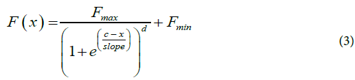
Once the five optimal parameters are obtained by fitting, they are then used within Eq.4 to determine the Cy0 value. The Cy0 value is the intersection between the x axis and the tangent of the Richards curve at the inflection point.
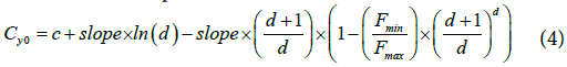
Cy0 can thus be computed for each sample and their ratio or rank used for comparison.
Logistic 5p Method: In [7], the curves are fitted with a logistic (Eq.5) five-parameter equation model in which the fifth parameter f models for a possible asymmetry of the sigmoid (Supp. Figure 3). However, both models fail to obtain a reliable F0 by setting x to zero in the fitted equation. Instead, the authors used the obtained parameters to estimate the efficiency of the reaction at the cycle of maximal second derivative using Eq.6. The authors extrapolated the value of F0 from an exponential model using these parameters and Eq.7.
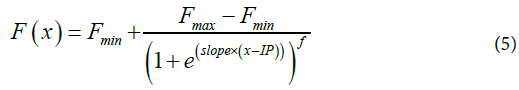
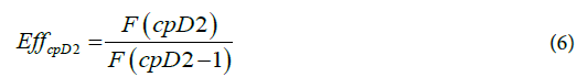
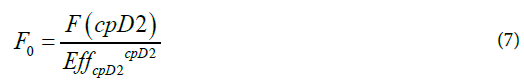
F0 can thus be computed for each sample and their ratio or rank used for comparison.
LRE method. A quantification method, SCF, was proposed by Liu and Saint [14] and then revised by Rutledge [8]. It finally became the LRE method [11]. In this approach, an estimated F0 is computed at each cycle within a window located in the lower amplification region of the curve using Eq.8 and Eq.9 :
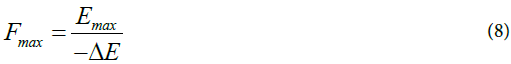
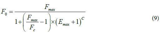
where Emax is the maximum efficiency of the reaction and ΔE its decreasing rate. An average F0 can thus be computed for each sample and their ratio or rank used for comparison.
Linreg Method: In [9], fluorescent values of a reaction are logged and a window of linearity is identified. From this window the efficiency and the N0 can be computed. In practice, implementing the LinReg method is unstable, since locating the window of linearity lacks robustness on real data. Indeed, in practice, despite our effective background correction, the second maximum derivative needed for this step was not systematically found within the exponential phase as expected in principle by the method. Importantly the authors acknowledge difficulties in going high throughput: “visual inspection of all amplification curves remains necessary in order to identify deviating samples that require an individual window or that may have to be excluded.” In our hand, full automation of LinReg proved to be impossible.
Deep Learning: Since qPCR kinetics seem difficult to fully apprehend, we tested a deep learning approach. We used one of the two datasets to train and test our model and used the other for validation. On each plate, all conditions for 3 genes were left out for testing purposes, and all the other conditions were used for training. Our deep learning model attempted to regress the logged theoretical initial copy number from the 40 fluo values. We used the Keras [15] framework and built a small neural network made of 2 hidden layers: a convolutional layer of kernel size 5 followed by a fully connected layer, in order not to over parameterize the function. We used the Adam optimizer, the Mean Squared Error as a loss function and a batch size of 128 curves as input. We trained the model over 20.000 epochs but the loss graph (Supp. Figures 4 and 5) revealed that 2.500 epochs were sufficient and also more precise in terms of genericity. This is thus the trained model we eventually used (Supp. Figure 6). With 40 fluorescent values given to this model as input for each sample, a predicted copy number can be output and the ratio or rank of these values between samples can be used for comparison.
Methods comparison
The datasets we use for comparison consist of two plates. In “Plate no. 1”, the initial copy number is only known for a subset of wells, whereas in “Plate no. 2”, the initial copy numbers are known for every well. Overall, we only used the wells for which the ground truth is known and no preamplification steps were performed prior plating, in order to limit biases. This sums up to 176 conditions (a 11-fold dilution of 16 genes) in sextuplicates on “Plate no. 1” and 352 conditions (a 11-fold dilution of the same 16 genes for PS and PC samples) on “Plate no. 2”. After identification and removal of flat curves with the approach we described earlier, we only considered sigmoidal curves for comparison. For “Plate no. 1”, this selection process ended up with 568 usable curves. To consider only robust data, we further discarded a few condition sextuplicates when at least one of the replicates did not exhibit a sigmoid profile. Overall, we retained 534 curves in 89 conditions. For “Plate no.2”, we discarded Notch1a gene in all samples and Crabp2a and BMP4 genes in PC samples due to uncertainties concerning their theoretical N0. Identification and removal of flat curves ended up to 1.120 curves, and further discarding all condition replicates when at least one of the sextuplicates did not exhibit a sigmoid profile, ended up in 894 curves in 149 conditions.
In practice, in our experience, replicates are rarely performed for high throughput qPCR experiments, as measurements are fairly reproducible. In this experiment, we nevertheless performed sextuplicates in order to assess variability, to compare methods with precision on the one hand, and to estimate the LOD as a function of preamplification cycles on the other hand. We compared the methods in four different ways in order to better understand the pros and cons of each approach in a high throughput setup. When comparing methods, the two main aspects we found important to monitor were: 1) their capacity to properly rank samples, because this is often the primary goal of an experiment, and 2) their capacity to retrieve the original gene copy log ratio difference between samples, since what is being sought is not only the right rank but also the right difference between samples. These two aspects were monitored by four metrics [16-18].
Metric 1: Absolute Log Ratio Difference Distribution. The distribution of absolute difference between the known gene copy (theoretical N0) log ratio for two samples S1 and S2 and the log ratio of measures between these samples provided by a given method. It quantifies the amplitude of the method deviation from the ground truth (Figure 2A).
Metric 2: Percentage of Proper Pairwise Ranking. The percent of correct ranking of measures between S1 and S2 provided by a given method (that is S1 < S2 or S2 < S1) as compared to the known gene copy (theoretical N0) rank between two samples S1 and S2. Note that the Cq method can return the same (integer) cycle result for different samples and since only the expected ranking is considered correct, ties are considered wrong. This metric counts the amount of ranking error (Figure 2B) as it is often the primary goal of an experiment: evaluating if a gene expression has increased or decreased between two conditions.
Metric 3: Replicates Coefficient of Variation. The coefficient of variation is computed from the sextuplicates available for each sample. The coefficient of variation is preferred to the standard deviation to limit the effect of the amplitude difference between output of each method (F0, Cy0, Cq, N0,..). This metric evaluates the method reproducibility for the same condition (Figure 2C).
Metric 4: t-test Between Sextuplicates. A t-test between groups of sextuplicates for each couple of conditions (Figure 2D). This metric encompasses metric 2 and 3 simultaneously by evaluating if the variation between replicates is small enough to detect a difference in gene copy numbers. The result is considered either correct (i.e. significantly different and ranked in the right order), undetermined (i.e. not significantly different) or wrong (i.e. significantly different but ranked in the wrong order) with an alpha level of 0.05. To obtain a closer understanding of how well the method fits, the possible comparisons were divided into 3 Groups:
• Group 1, “Large differences”: theoretical log ratio greater than 2 (n=2.391)
• Group 2, “Intermediate differences”: theoretical log ratio between 0.2 and 2 (n=2.571)
• Group 3, “Subtle differences”: theoretical log ratio less than 0.2 (n=662)
Results
A Robust Curve Fitting Method Adapted to High Throughput qPCR
In order to compare data analysis approaches, we ought to properly fit thousands of samples from our high throughput experiments to all parametric models proposed. However, stochastic optimization performed automatically for thousands of curves necessarily results in numerous fitting failures. This is mainly due to the fact that parameter search is often initialized randomly, thus far from the global optimum. In order to avoid this, we developed a dedicated fitting procedure (Figure 1). Our approach takes advantage of the throughput to initialize parameters as closely as possible to the best local minima, so as to ensure that the optimization process converges toward the global minimum. It relies on the hypothesis that the ~10.000 curves of a typical high throughput qPCR plate encompass a limited set of shapes that can be roughly described as a set of clusters on the parameter space.

Figure 1: (A) A massive parallel regular fitting on a high throughput dataset results in a large fraction of curve fitting failure due to inadequate random initialization of the parameters. (B) A subset of curves are randomly fitted and a clustering step identifies k spreaded locations in the parameter space covering close approximations of all possible curves. (C) Non random parameter initialization by the k centers results in a robust fitting of all curves.
As a preprocessing step, initial parameter sets were randomly sampled within relevant ranges and the fitting parameters were obtained through parallel minimization of the mean square error on a random subset of curves (~1.000). As expected, many fitting attempts failed in this first trial. However, parameter vectors obtained from the successful fits were further normalized and considered in a clustering step using a simple k-means. The k classes thus obtained described a close approximation of all the possible curves one might encounter in such a dataset. The k-centers of these classes could then be used as k initial parameter sets to fit all the curves in the dataset with two interesting properties. First, k was a small number (typically lower than 10) which made tractable the fitting of tens of thousand curves in a reasonable time on a regular computer. Secondly, given the clusters covered all possible curves, it ensured that at least one of the k-centers was already close to a good if not optimal solution. From this point, it was then sufficient to attempt k fit initialized by the k-centers on each curve and to choose the one minimizing the error among them. In practice, it is permitted to obtain an accurate fit for tens of thousands of curves in a row without optimizer divergence.
We designed and performed an objective comparison of available qPCR data analysis methods when ported to high throughput. Importantly, output of the method tested could not be directly compared, as they do not carry on the same information. For instance, Cq relates directly to the cycle, while F0 produced by LRE or the logistic5p is the theoretical estimated fluorescence value at cycle 0 that can be transformed into a molecule count through optical calibration. Furthermore, deep learning approaches don’t have to use this calibration step but do need a large training set with known initial amounts to directly produce a molecule count. For these reasons, we boil down the comparison to the final outcomes that are expected from the analysis of such a high throughput qPCR experiment: Are any two samples properly ranked in terms of gene copy number? Is the amplitude of the difference between these two values properly retrieved? Is the measure robust?
On all of the four metrics (see methods), the Cq method performed the best by providing on average the most accurate results, with the Cy0 method being almost as good. While depending on a training dataset, the deep learning approach also seemed to perform well (Figure 2B-D). In all metrics, 5p and LRE are outperformed with a lower accuracy on the log ratio compared to the ground truth (Figure 2A) and higher replicates coefficient of variation (Fig -ure 2C). Note that most methods properly rank 80% of the samples because the initial amount of some of these samples is highly different. Therefore, in order to distinguish obviously different quantities from intermediate amounts and samples displaying subtle differences, we split the samples into three groups (Figure 2D). While the Cq method performs best on intermediate amounts, Cq, Cy0 and deep learning could barely be decided, as they produce errors of different kinds on subtle differences of initial gene copy number.
Discussion
To our knowledge, no study currently exists to compare qPCR data analysis methods when ported to high throughput. One reason for this may be that there was no method developed for low throughput data that was readily or easily portable to high throughput experiments. Indeed, porting low throughput methods to high throughput data analysis can encounter several difficulties. For instance, if a method used to require a user input for each sample it would become a critical issue. This input can take different forms such as choosing a threshold, selecting a set of cycles, etc. Among the ones we tested, LRE and LinReg methods seemed to be the one that suffers automation the most. In the case of LinReg, we simply didn’t succeed to port it to high throughput. As for LRE, the authors acknowledged that a user intervention might be needed to choose the starting point of the linear window to consider to regress efficiency. In the original paper, the author suggests choosing it within the lower region of the amplification profile, an instruction not straightforward to automate. In a further revision. Rutledge proposed choosing the cycle where fluorescence reaches half of its maximum, acknowledging that it is suboptimal and could be refined by hand if desired. In our hand, we weren’t able to automatically find a “universal” starting point that was fully satisfactory for all curves and thus producing the output accuracy claimed at low throughput by the authors. Actually, this choice has an important impact on the computation of efficiency and thus on the F0 value. In the same way, for the logistic5p method, we encountered two issues. In the log-logistic equation Eq.5 was preferred over the logistic, but we had to use the latter, because the parameter sensitivity of the former induced a large number of fitting divergence, despite the robust fitting method we proposed. Moreover, in our case, we derived the second derivative from the fitted model, rather than the raw data as specified in the original paper, so as to avoid the plateau effect and make the measure more robust, for otherwise many curves would not have produced a relevant value. Overall, all methods required an adaptation to be ported to high throughput without which they couldn’t have been tested.
Whatever the method used, background removal had to be performed and it looked like the unexplained background signal didn’t display a unique pattern. This sort of bias is related to factors such as the chemistry and device used or the batch. It does however seem reasonable to deal with background removal in a data analysis in an independent fashion. We choose to make it independent of the quantification method itself but it could be interesting to merge both steps. For instance we observed that the deep learning approach performed almost as well without background correction because these factors were also learnt and cancelled out by the model.
The literature and most of the methods presented here consider efficiency as being a parameter that can be defined, extracted and used to estimate the number of copies in the original sample. However, its definition itself is debated: some as in LRE consider that this efficiency varies over time, others consider that the efficiency is fixed per gene, per condition or per reaction... It thus makes sense that its computation has divided the community for a long time. Each of the Logistic5p and LRE methods suggests a way to compute the efficiency to obtain the F0 value. In our hand, because it is ill-defined and variable, we found that its determination was very sensitive and led to errors that were especially obvious on the metric 1 (Figue 2A). Overall, we concluded that the efficiency is sample and cycle dependent and that it didn’t make things easier to attempt to explicitly evaluate it in order to reach the final objective: comparing samples.
Overall, Cq and Cy0 methods seem to be the most accurate methods. However, in practice, Cy0 method is very easy to set up. This modified standard curve-based method does not require assumption of uniform reaction efficiency between curves, does not involve any choice of threshold level by the user and does not imply any reference gene. It’s perfectly adapted to automated high throughput data analysis since it’s based on a fitting and computation on the optimal fitting parameters. Though it is not the method that provides the best results, it doesn’t show any particular weakness over the 3 first metrics (Figure 2A-C). Regarding the 4th (Figure 2D), most complete one, it shows a remarkably low undetermined rate, though, as for all methods, on the group 3 comparisons, it has almost as much wrong results as correct ones.

Figure 2: Comparison of qPCR data analysis methods when ported to High throughput
Top to bottom and left to right. A) The distribution of the pairwise sample absolute log ratio difference to compare how close/far are the results obtained by a given method to the ground truth. (B) Percentage of correct pairwise sample ranking per method. (C) Replicate samples coefficient of variation per method. (D) Replicate samples t-test to determine whether the gene/condition sextuplicates pairs are correctly ranked in regard to the closeness of the initial quantities.
The different methods were compared using two datasets we produced from the same machine and chemistry but with a threeyear shift and done by two different people. It makes a reasonable dataset with thousands of samples but some of the conclusions we draw here could be challenged with additional datasets produced on other platforms. For instance, some methods could be more adapted to a specific chemistry. For example, Rutledge acknowledges that the LRE method was not extensively tested on TaqMan. In order to improve both the method and the comparison, we provide the scientific community with the code of the methods and our datasets with the known initial molecule amount per well.
The robust fitting method we propose requires three input parameters: the number of curves randomly selected to determine a relevant set of initial fitting parameters (in practice a thousand), the number of fitting trials for each of these curves (in practice a hundred) and, finally, the number of clusters designating the number of initial parameter sets (in practice a dozen), or equivalently the number of different curve types we roughly expect. In practice, the results were robust to the variation of these parameters on our own datasets with all nine thousand curves of a plate being always successfully fitted. Therefore, we anticipate that the approach should remain robust when applied to other datasets because of its core principle: it scans all possible curve shapes, identifies their parameters and uses them as initial parameters to subsequently fit all the curves of a plate. Beyond HT-qPCR, the fitting protocol presented here could be directly applied to other types of applications whenever high throughput fitting is required.
An advantage of the deep learning approach we observed was that it did not require the background removal preprocessing step. Indeed, not using it didn’t degrade the results significantly. However, we had expected that deep learning could decipher qPCR hidden features better than the regular methods. Our finding is that qPCR sigmoid curves exhibit a rather simple model that doesn’t need a very sophisticated neural network to be captured since for each curvethe cycle values are highly correlated. In effect, the spectrum of the possible functions that relate cycle value to fluorescence is rather narrow. In practice, the deep learning model we created and trained ended up not being very deep since increasing the amount of parameters simply led to overfitting. Furthermore, we were limited to performing a training on the data available to us for which we had designed a way to produce ground truth, but a well known weakness of machine learning is that it depends on a training dataset that necessarily includes bias. Therefore, we cannot assume that the training we perform could be used as such to evaluate data obtained from another experimentalist, from another device and/or another chemistry. We could even hypothesize that it would yield poor results.
Conclusion
Altogether, we presented an objective quantitative comparison of data analysis methods for high throughput qPCR data. 6 methods were compared (Cq, Cy0, logistic5p, LRE, LinReg and deep learning) using four metrics on two high throughput datasets with known ground truth. The results indicate that LinReg could not be ported to high throughput and that logistic5p and LRE produced less accurate results than Cq, Cy0 and deep learning. Among these last three, the simplest method, Cq, was also slightly more accurate at retrieving the actual difference between samples. We therefore conclude that Cq should be preferred over more complex methods for high throughput qPCR data analyses.
Code Availability
Custom scripts that were used for this study are available at: https://github.com/biocompibens/qPCR.
Data Availability
Data corresponding to the two high throughpout qPCR plates used in this study are available at: https://doi.org/10.7910/DVN/ NDSN5W
Conflicts of Interest
Authors declare no conflicts of interest
Acknowledgements
We thanks Mary Ann Lettellier for valuable comments on the manuscript. This work has received support under the program «Investissements d’Avenir» launched by the French Government and implemented by ANR with the references ANR–10–LABX–54 MEMOLIFE and ANR–10–IDEX–0001–02 PSL* Université Paris.
References
- Saiki RK, Scharf S, Faloona F, Mullis KB, Horn GT, et al (1992) Enzymatic amplification of beta-globin genomic sequences and restriction site analysis for diagnosis of sickle cell anemia. Biotechnology 24:476–480.
- Pabinger S, Dander A, Fischer M, Snajder R, Sperk M, et al (2014) A survey of tools for variant analysis of next-generation genome sequencing data. Brief Bioinform 15:256–278.
- Higuchi R, Fockler C, Dollinger G, Watson R (1993) Kinetic PCR analysis: real-time monitoring of DNA amplification reactions. Biotechnology 11:1026–1030.
- Baker M (2010) Clever PCR: more genotyping, smaller volumes. Nature Methods 351–356.
- Spurgeon SL, Jones RC, Ramakrishnan R (2008) High Throughput Gene Expression Measurement with Real Time PCR in a Microfluidic Dynamic Array. PLoS ONE1662.
- Guescini M, Sisti D, Rocchi MBL, Stocchi L, Stocchi V (2008) A new real-time PCR method to overcome significant quantitative inaccuracy due to slight amplification inhibition. BMC Bioinformatics 9: 326.
- Spiess A-N, Feig C, Ritz C (2008) Highly accurate sigmoidal fitting of real-time PCR data by introducing a parameter for asymmetry. BMC Bioinformatics 9: 221.
- Rutledge RG (2004) Sigmoidal curve-fitting redefines quantitative real-time PCR with the prospective of developing automated high-throughput applications. Nucleic Acids Res 32:178.
- Ramakers C, Ruijter JM, Deprez RHL, Moorman AFM (2003) Assumption-free analysis of quantitative real-time polymerase chain reaction (PCR) data. Neurosci Lett 339: 62–66.
- Livak KJ, Schmittgen TD (2001) Analysis of relative gene expression data using real-time quantitative PCR and the 2- ΔΔCT method. Methods 25:402–408.
- Rutledge RG (2011) A Java program for LRE-based real-time qPCR that enables large-scale absolute quantification. PLoS One 6:17636.
- Marusic M, Bajzer Z, Freyer JP, Vuk-Pavlovic S (1994) Analysis of growth of multicellular tumour spheroids by mathematical models. Cell Prolif 27:73–94.
- Ruijter JM, Ramakers C, Hoogaars WMH, Karlen Y, Bakker O (2009) Amplification efficiency: linking baseline and bias in the analysis of quantitative PCR data. Nucleic Acids Res 37:45.
- Liu W, Saint DA (2002) A new quantitative method of real time reverse transcription polymerase chain reaction assay based on simulation of polymerase chain reaction kinetics. Anal Biochem. Available from: http://www.gene-quantification.net/liu-saint-1-2002.pdf.
- Keras Team (2001) Keras: the Python deep learning API. Available from https://keras.io/
- Panina Y, Germond A, David BG, Watanabe TM (2019) Pairwise efficiency: a new mathematical approach to qPCR data analysis increases the precision of the calibration curve assay. BMC Bioinformatics 20: 295.
- Rebrikov DV, Trofimov DY (2006) Real-time PCR: A review of approaches to data analysis. Appl Biochem Microbiol 42: 455–463.
- Rutledge RG, Stewart D (2008) A kinetic-based sigmoidal model for the polymerase chain reaction and its application to high-capacity absolute quantitative real-time PCR. BMC Biotechnol 8: 47.