Spanish
  Chinese
  Russian
  German
  French
  Japanese
  Portuguese
  Hindi
Hindi Research Article, J Soil Sci Plant Health Vol: 1 Issue: 1
Soil Survey: Prediction of Sum of Bases Using K-Nearest Neighbor Approach
Cathy A Seybold*, Moustafa Elrashidi and Zamir Libohova
USDA-NRCS (National Soil Survey Center), 100 Centennial Mall N., Rm. 152, Lincoln, NE 68508, USA
*Corresponding Author : Cathy A Seybold
USDA-NRCS (National Soil Survey Center), 100 Centennial Mall N., Rm. 152, Lincoln, NE 68508, USA
Tel: 402-437-4132
Fax: 402-437-5336
E-mail: cathy.seybold@lin.usda.gov
Received: August 14, 2017 Accepted: August 15, 2017 Published: August 22, 2017
Citation: Seybold CA, Elrashidi M, Libohova Z (2017) Soil Survey: Prediction of Sum of Bases Using K-Nearest Neighbor Approach. J Soil Sci Plant Health 1:1.
Abstract
In soil survey there is no pedotransfer function available to estimate sum-of-bases (SBs) for the range of soils that occur in the United States. The objectives of this study were to develop a SBs model using the k-nearest neighbor (k-NN) approach and validate this model against an independent dataset. The nearest-neighbor approach passively stores the development (or reference) dataset until the time of application, and then the dataset is searched for the 10 (k) most similar soils to that of the target soil, based on selected attributes (i.e., OC, cation exchange, pH, extractable acidity). The reference dataset was developed from the National Cooperative Soil Survey characterization database in Lincoln, Nebraska. Taxonomic order is used as strata within the reference dataset. The overall model prediction error (or RMSEp) was 2.104 cmol (+) kg-1 with a ME of -0.15 cmol (+) kg-1. Among the soil order groups, the RMSEp ranged from 1.169 to 5.943 cmol (+) kg-1, with the Histosols order having the largest RMSEp. Because of the underrepresentation of organic layers (compared to mineral layers) in the reference database, prediction errors tend to be higher. The overall low prediction errors suggest that the four properties (i.e., cation-exchange, pH, extractable acidity, and organic carbon) were effective in finding the nearest soils (to the target soil) in the reference dataset. In soil survey, the k-NN SBs model provides an efficient and reasonably accurate tool for estimating sum of bases (up to 100% base saturation) when measured data are not available for soils of the US.
Keywords: Sum of bases; Base saturation; Prediction; Soil survey; k-Nearest neighbor model
Introduction
Sum of bases (SBs) as defined here are the sum of extractable bases (i.e., Ca2+, Mg2+, K+, and Na+) determined with ammonium acetate (1N NH4OAc) buffered at pH 7, reported on <2 mm base with units of cmol(+) kg-1. Sum-of-bases is used in the calculation of base saturation, which is the percentage of the soil exchange complex occupied by base cations [1]. It is a measure of inherent fertility. Generally, soils with a high percent base saturation have higher soil fertility. Soils in the pH range 5.5 to 7.0 or 8.2 generally have a measured base saturation of less than 100 percent. Base saturation values are particularly low for weathered soils dominated by minerals such as kaolinite, which has a high proportion of pH-dependent charge [2]. Below pH 5.5, exchangeable Al saturation increases, and the exchangeable base saturation decreases with decreasing pH [1]. Base saturation is used as a criterion in Soil Taxonomy, separating Mollic (high base saturation) from Umbric (low base saturation) epipedons [3]. Base saturation is used as a criterion for Ultisols, Ultic subgroups of Alfisols, Andisols, and Mollisols, Alfic and Dystric subgroups of Inceptisols, and Alfic subgroups of Spodosols [4]. Sum of extractable bases is used directly as a criterion to classify soils in most of the Eutric subgroups of Andisols.
Sum of bases (SBs), from which base saturation is derived, is a soil property that is captured in the National Soil Information System (NASIS) database of the USDA-NRCS for soil map unit components (i.e., soils/series that make up the map unit). There are no field estimation methods available [4]. Measuring SBs is not practical everywhere and at every depth within all map unit components in a survey area or for an update. Predictive models become useful in these cases, which are based on soil descriptions and other more easily obtained data existing in the soil survey database. However, given the need, there are no national soil survey guidelines or models for estimating SBs [4]. There is no national model for estimating SBs. There are still areas where initial soil mapping is occurring and there are many areas going through updates, especially on an MLRA basis. To improve estimates of SBs, a model that is national in scope and uses available properties within the soil survey database is needed.
Soil pH has been commonly used to estimate base saturation when laboratory data are not available [5,6]. However, it was pointed out by Thomas and Hargrove [7] that the relationship between pH and base saturation can differ greatly from soil to soil. Ranney et al. [8] developed SBs prediction equations for northeastern Pennsylvania from 555 soil profiles using pH, moisture surplus and drainage class as independent variables. They found percent moisture content to be higher at a given pH in areas of low total moisture surplus and in areas of poorer drainage. Gray et al. [9] using the ISRIC WISE Global database, developed broad relationships between SBs and the soil forming factors using three different modeling approaches. In their regression model approach, variables significant in their prediction of SBs were parent material, climate, and slope. Aitkenhead et al. [10] developed a Neural Network model using the National Soil Inventory of Scotland (NSIS) to predict several parameters, one of them being sum of exchangeable bases. Their input parameters corresponded closely to the soil forming factors and human influence, and SBs was categorized as being well predicted with an r2 = 0.56. Genu and Dematte [11] found it possible to estimate SBs for a specific region in Brazil using infrared spectral data, which were comparable to multiple regression estimates. Nettleton et al. [12] developed a multiple regression model for predicting base saturation for Andisols with predictor variables of pH in water, clay content, and pH in NaF (r = 0.92; SE = 11.2). In summary, there are only a few models that have been developed, and they are specific to a region or country or to a specific type of soil and would not be applicable to the wide range of soils that occur within the U.S.
A nonparametric approach, called k-nearest neighbor (k-NN), was used by Nemes et al. [13] in the prediction of water contents at 33 kPa and 1500 kPa matric potentials and by Seybold et al. [14] in the prediction of bulk density. The k-NN approach belongs to a group of “lazy learning algorithms” in which the model passively stores the development data set until the time of application. All calculations are then performed when an estimation of the property is generated. This involves identifying and retrieving the nearest stored values (k) relative to the unknown or target soil. The k-NN approach could be well suited to the prediction of SBs because a large soil survey characterization database containing thousands of measured values from all across the U.S. is available along with pedological information.
The objectives of this study were to develop a model to predict SBs using the k-NN approach and validate the model against an independent dataset. The model would be limited to the basic soil properties captured in soil survey that are related to SBs such as pH and taxonomic classifications. A prediction model, that is national in scope, will provide consistent and improved accuracy of SBs estimates, which will benefit all users of soil survey data and their interpretations as soil survey data is being updated or through initial mapping.
Materials and Methods
Soil data
Measured data were selected from the Kellogg Soil Survey Laboratory (KSSL) database in Lincoln, NE. This database contains over 37,000 pedons with measured chemical and physical data, representing geographically diverse soils from across the conterminous U.S., Hawaii, and Alaska. The following measured data were used from the database: total sand (2-0.05 mm), total silt (0.05-0.002 mm), and total clay (< 0.002 mm) (pipette method), organic C content (acid-dichromate digestion method, discontinued in 2000), total C (dry combustion), CaCO3 equivalent (electronic manometer method), gypsum content (<2 mm), electrical conductivity (saturated paste method), cationexchange capacity (CEC) (1.0 N NH4OAc at pH 7), effective cationexchange capacity (ECEC) (1.0 N NH4OAc at pH 7), pH (in water and in CaCl2), sum of extractable bases (NH4OAc, pH 7.0), and extractable acidity (barium chloride-triethanolamine, pH 8.2). All methods are described in Soil Survey Staff [15]. Most determinations were from airdried (30-35°C), crushed, and sieved (<2 mm) soil samples. Data are reported on an oven-dry basis. Other data used were the soil taxonomic classifications from the soil’s profile description. Base saturation was calculated from SBs by dividing SBs by the CEC or ECEC and multiplying by 100. Sum of base values were corrected to 100% base saturation in cases when the extractable bases were greater than 100% base saturation. This occurs when there are soluble salts, gypsum and carbonates present in the soil, which contribute bases in the extract [15]. Where total C was measured, the organic carbon was determined by difference between the total C and CaCO3-C [1].
The measured data was split into a development dataset and a validation dataset. Because of the nature of this model, most of the data was used for model development (88%). A reference dataset that is to be used by the k-NN model was developed using the development dataset. Figure 1 shows the locations of the pedons used in the reference (or development) dataset (conterminous US only). Selection of attributes (or input parameters) to include in the reference dataset was based on what others have used in predicting SBs or base saturation, and evaluating relationships between base saturation and soil properties. Pearson correlations were computed to evaluate these relationships. To evaluate categorical variables as input variables (such as taxonomic order, mineralogy class and master horizon designation), effects coding in general linear models was used to produce parameter estimates that are differences from group means [16].

Figure 1: Sample location of pedons (continental US only) that make up the reference dataset used in the prediction of sum-of-bases.
K-Nearest neighbor (k-NN) approach
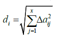
The k-NN approach was first described by Nemes et al. [13] in the prediction of water contents at 33 and 1500 kPa matric potentials, and was later applied by Seybold et al. [14] in the prediction of bulk density using their approach. For the convenience of the reader, the k-NN approach as summarized in Seybold et al. [14] is presented here. There are no predefined mathematical functions that estimate SBs. A “reference dataset” is searched for soils that are most similar to the target soil, based on selected attributes (e.g., pH, CEC, and OC). The “distance” (a measure of similarity) of each soil to the target soil (in the reference dataset) is calculated:
 (1)
(1)
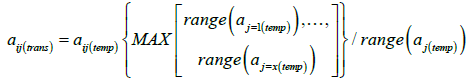
Where di is the distance of the ith soil from the target soil, and Δaij is the difference of the ith soil from the target soil in the jth soil attributes [13]. In the present study, there are more than two input attributes (e.g., CEC, OC, and pH), so the attribute values are normalized before they are used to calculate “distance”, which avoids bias towards one or more attributes [13]. As a result, temporary variables are generated with a distribution having a zero mean and a standard deviation of one using the following transformation from [13]:
![]() (2)
(2)
Where aij represents the value of the jth attribute of the ith soil, and ÄÂj and σ(aj) represent the mean and standard deviation of the observed values of the jth attribute in the reference data set. Then, the minimum-maximum range of those temporary variables, are scaled to obtain zero mean and the same minimum-maximum range in the data of all attributes:
 (3)
(3)
Where aj(temp) represents the data of the jth soil attributes normalized using Eq. 2; and aij(trans) represents the final transformed value of the jth attribute of the ith soil that are to be used as input [13]. It should be noted that taxonomic order is a strata within the reference dataset and was not normalized. Within soil order the continuous attributes were normalized.
The closest 10 soils (k) in the reference dataset (within the soil order strata) were then used to formulate the estimate of the output SBs. It was shown by Nemes et al. [13] that k was not very sensitive to reference data set size as long as k was above 8 or 9 (in their particular case). A k of 10 was successfully used in a k-NN model for predicting soil bulk density [14]. We felt there was no reason to alter k; therefore a k of 10 was used here in the present study.
Nemes et al. [13] presented the argument that a soil closer to the target should have more weight in calculating the estimated value. Therefore, their distance-dependent weighting system was employed here to account for the distribution of the distances of the selected 10 nearest soils to the target:
 (4)
(4)
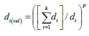
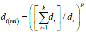
Where k is the number of neighbors considered, and wi is the assigned weight, and di(rel) is the relative distance of the ith selected neighbor, calculated as:
 (5)
(5)
Where k is the number of neighbors considered, and di is the distance of the ith selected neighbor calculated using Eq. 1, and p is a power term that was set to one for the estimation of SBs in the present study. Nemes et al. [13] has shown that p values remained around one and were generally insensitive to sample size (in their particular case), suggesting that “one” is a safe first approximation. Attribute weights were applied equally across the entire data space. The final result was average weighted SBs of the 10 nearest soils within taxonomic order strata in the reference dataset.
Model development
The k-NN model for predicting SBs was programmed as a “Calculation” in the National Soil Information System (NASIS) (version 6.4). The scripting language in NASIS for Calculations, Validations, Interpretations and Reports (CVIR) uses a variant of the Structured Query Language (SQL) [17]. The result of the calculation can be set in the database. The reference dataset is called into the model as an “input” file. The model is available as a choice and can be used by the soil scientist when no measured data are available and when an estimate is needed, when populating or updating the NASIS database for a mapunit component.
Validation
The SBs k-NN model was validated with an independent dataset of measured properties from the KSSL database, consisting of 4,347 horizons. The soil horizons represented pedons from all across the United States, including Alaska and Hawaii. Measured versus predicted SBs was evaluated using the general linear model procedure in SYSTAT [16]. Confidence intervals (95%) were calculated for the slope and intercept of the least square estimate line. Performance measures were the root mean square error (RMSE) and mean error (ME) as calculated in McBratney et al. [18]. The RMSE gives the accuracy of the estimations in terms of standard deviation.
Results and Discussion
Application of the k-NN technique requires identification of input parameters that will be used to find soils nearest to the target soil [13]. Correlation of soil properties with base saturation were evaluated for this purpose. Soil pH in water had the highest correlation to the base saturation (r=0.77). Base saturation generally decreases with lower pH values. Beery and Wilding [5] have also shown a relationship of pH to base saturation for Ohio soils. They found pH to be a more reliable predictor in surface soils than that in subsoils at predicting base saturation. In the present study, extractable acidity had a moderately negative correlation with base saturation (r=-0.45). This would be expected, as exchangeable Al3+ and H+ increase, the exchangeable bases would decrease on the exchange complex. Effective cation exchange capacity and CEC had weaker correlations with base saturation (r = 0.36 and r = 0.10, respectively). Pierre and Scarseth [19] in soils of like pH values also found imperfect correlations of CEC with base saturation. Organic carbon does have cation-exchange properties, which also had a weak negative correlation with base saturation (r=-0.19). In a study by Blosser and Jenny [20], correlations of base saturation with soil properties were improved when soils were grouped into classes based on OC and CEC. By grouping in this manner, they were able to control the soil forming factor of climate. They postulated that control of soil forming factors should improve correlations among soil properties with base saturation. Based on their conclusion and correlations in the present study, OC and CEC where selected as input parameters for inclusion in the reference dataset. There was no other soil property that showed any significant relationship to base saturation. Because the above four properties (i.e., cation-exchange, pH, extractable acidity, and OC) have some relationship to base saturation (directly or indirectly), they were selected as input variables that will be used to find the 10 closest soils (to the target soil) in the reference dataset. Additionally, both CEC and ECEC were included because in our soil survey database (NASIS) CEC is only available for soils with pHs>5.5 and ECEC is available for soils with pHs ≤ 5.5. Similarly, in NASIS, pH in water is available for mineral soils and pH in CaCl2 is available for organic soils. To build a model for all soils, both pH data and cation exchange data (CEC and ECEC) must be included as input variables in the reference dataset. Different input parameters will be used depending on the target soil’s available properties.
Taxonomic order is the broadest category in soil taxonomy and is based largely on soil-forming processes as indicated by the absence or presence of major diagnostic horizons, which are defined and separated based, in part, on base saturation [3]. Thus, a given order includes soils whose properties (including base saturation) suggest that they are somewhat similar in their genesis. We tested soil order to determine if it would be useful as an input variable. Soil taxonomic order alone was able to explained 48% of the variation in base saturation (r2 = 0.48). Therefore, soil order was included as an input parameter in the reference dataset. The soil properties of the target soil would be matched to the properties within the same soil order in the reference dataset. Soil taxonomic mineralogy class and master horizon designation were also considered, but were only able to explain an additional 2% of the variation in base saturation when included with soil taxonomic order (r2=0.50). Within the soil orders in the reference dataset, organic layers are underrepresented. Therefore, organic layers were separated from the soil orders and combined into their own group. Combining the organic layers into their own group increased a searchable group to 170 layers if CEC is an input variable and 91 layers if ECEC is an input variable (Table 1). The reference dataset will be searched for the k most similar soils (the closest soils) to the target soil within the same taxonomic order or the organic soil group (Table 1). Also, because some soil orders (i.e., Histosols, Gelisols, Aridisols, and Vertisols), mostly for layers with pHs<5.5, are underrepresented (n<70) in the reference dataset, they were grouped with other soil orders. Histosols, Gelisols, and low pH Aridisols were combined with Inceptisols, and low pH Vertisols were grouped with the Alfisols (Table 1). Also, soil horizons that have hydrous, medial, or ashy texture modifiers in soil orders other than Andisols were grouped with the Andisols (Table 1). Andisols and layers with andic soil properties (typically formed during weathering of volcanic materials) will have properties that vary greatly from other soils [21].
| Taxonomic Order or Organic Group | Description | N | |
|---|---|---|---|
| Organics | OC contents > 14.5% | CEC | 170 |
| ECEC | 91 | ||
| Andisols | Includes layers of other orders with ashy, medial or hydrous in-lieu-of textures | CEC | 916 |
| ECEC | 653 | ||
| Ultisols | Ultisols with = 14.5% OC | CEC | 783 |
| ECEC | 3,065 | ||
| Oxisols | Oxisols with = 14.5% OC | CEC | 314 |
| ECEC | 710 | ||
| Inceptisols, Gelisols (65), Histosols (135) | Inceptisols, Gelisols, and Histosols with = 14.5% OC, includes low pH layers of Aridisols (26)† | CEC | 2,429 |
| ECEC | 2,435 | ||
| Spodosols | Spodosols with = 14.5% OC | CEC | 574 |
| ECEC | 1,647 | ||
| Alfisols | Alfisols with = 14.5% OC, includes low pH layers of Vertisols (68)† | CEC | 7,110 |
| ECEC | 4,704 | ||
| Entisols | Entisols with = 14.5% OC | CEC | 1,221 |
| ECEC | 578 | ||
| Mollisols | Mollisols with = 14.5% OC | CEC | 7,450 |
| ECEC | 621 | ||
| Vertisols | Vertisols with = 14.5% OC | CEC | 494 |
| Aridisols | Aridisols with = 14.5% OC | CEC | 651 |
†Number in parenthesis is the number of layers with the taxa (includes both high and low pH layers).
Table 1: Within the reference dataset, the target soil is matched to the closest soils within the same taxonomic order or organic group.
A SBs model was developed that determines SB values (up to 100% base saturation) for a wide range of soils that occur in the US. The model searches a reference dataset, and get the 10 (k) closest soils (to the target soil) within the same taxonomic order or organic group. The corresponding measured SBs are then weighted based on distance (or similarity) to the target soil and averaged (Figure 2). Within the model, the pH and OC content of the target soil will dictate whether CEC or ECEC is used and whether pH in water or pH in CaCl2 is used with OC and extractable acidity as input variables for a particular horizon.

Figure 2: Schematic overview of the k-nearest neighbor approach for predicting sum-of-bases.
Input parameters of the target soil needed by the model are taxonomic order [3], OC content, pH (in H2O or CaCl2), CEC or ECEC, and extractable acidity and whether gypsum and/or calcium carbonate are present. The model runs through a series of decisions regarding the target soil when finding the 10 nearest neighbors in the reference dataset. If the target soil contains gypsum or calcium carbonate, or the pH (in water) ≥7.5 then 100% base saturation is assumed [1,22], and the CEC value of the target soil is assigned as the SBs value. Next, if the organic C content of the target soil is > 14.5%, then OC, pH (in CaCl2), extractable acidity, and CEC or ECEC of the target soil are used to get 10 of the closest soils in the organics group in the reference dataset. Next, if the texture modifier is ashy, medial, or hydrous; then OC, pH (in water), extractable acidity, and CEC or ECEC of the target soil are used to get 10 of the closest soils in the Andisols order in the reference dataset. And for everything else the OC, pH (in water), extractable acidity, CEC or ECEC, and soil order of the target soil are used to get 10 of the closest soils within the same soil order in the reference dataset.
The reference dataset contains 36,910 layers of measured data that consist of CEC and ECEC, pH in water and CaCl2, organic carbon, extractable acidity, SBs and taxonomic order. For the reference dataset, basic statistics and ranges of the properties are presented in Table 2. Organic carbon ranges from 0 to 59%, which covers the whole range possible. Measured SBs ranges from <0.1 to 398 cmol(+) kg-1, which was corrected to the 100% base saturation (if greater). All 12 taxonomic soil orders are represented in the reference dataset.
| Property | N | Min | Max | Median | Mean | Std. Dev. |
|---|---|---|---|---|---|---|
| pH (H2O) | 36,910 | 2.1 | 10.1 | 5.7 | 5.8 | 0.9 |
| pH (CaCl2) | 33.838 | 2.2 | 9.4 | 5.2 | 5.2 | 0.9 |
| CEC (cmol(+) kg-1) | 36,910 | 0.1 | 196 | 13.8 | 16.5 | 13.2 |
| ECEC (cmol(+) kg-1) | 14,810 | <0.1 | 152 | 6.0 | 8.7 | 8.0 |
| Ext. Acidity (cmol(+) kg-1) | 36,910 | < 0.1 | 249 | 6.0 | 9.1 | 11.3 |
| Organic Carbon (%) | 36,910 | < 0.1 | 59 | 0.5 | 1.3 | 2.9 |
| Sum bases (cmol(+) kg-1) | 36,910 | < 0.1 | 186 | 8.2 | 11.4 | 11.3 |
Table 2: Ranges in soil properties of the reference dataset used to predict sumof-bases.
Validation
Performance of the k-NN model depends largely on the goodness of selection of the most similar (nearest) soils to the target soils [13]. The model was validated against an independent dataset consisting of 4,347 soil horizons. The validation data set consisted of a wide variety of layers from all 12 taxonomic orders. Measured SB values (corrected to 100% base saturation) ranged from 0.1 to 140 cmol(+) kg-1 and OC values ranged from 0.0 to 57 %. Statistical properties of the validation dataset are presented in Table 3.
| Property | N | Min | Max | Median | Mean | Std. Dev. |
|---|---|---|---|---|---|---|
| pH (H2O) | 4,347 | 3.0 | 10.0 | 5.8 | 5.9 | 1.10 |
| pH (CaCl2) | 4,347 | 2.7 | 9.8 | 5.2 | 5.4 | 1.14 |
| CEC (cmol(+) kg-1) | 2,612 | 0.1 | 143 | 15.3 | 18.1 | 14.1 |
| ECEC (cmol(+) kg-1) | 1,736 | 0.2 | 66.9 | 6.3 | 8.5 | 7.6 |
| Ext. Acidity (cmol(+) kg-1) | 4,101 | < 0.1 | 236 | 8.3 | 12.4 | 14.7 |
| Organic Carbon (%) | 4,347 | < 0.1 | 52.3 | 0.6 | 1.9 | 4.4 |
| Sum bases (cmol(+) kg-1) | 4,347 | < 0.1 | 140 | 7.7 | 11.2 | 11.9 |
| Gypsum (%) | 179 | < 0.1 | 51 | < 0.1 | 1.9 | 6.9 |
| CaCO3 (%) | 545 | < 0.1 | 98 | 1.0 | 9.8 | 17.8 |
Table 3: Ranges in soil properties of the validation dataset used to predict sumof-bases.
Measured versus predicted SB values (predicted up to 100% base saturation) are presented in Figure 3. There is general agreement between the measured and predicted SBs as indicated by the high r2 value of 0.97. The accuracy of the predictions produced an RMSEp of 2.104 cmol(+) kg-1 and an overall ME of -0.15 cmol(+) kg-1. Comparing our results with others who have predicted SBs have shown higher RMSEs and lower r2 (lower prediction accuracies). Gray et al. [9] using the ISRIC WISE Global database in the development of broad relationships between SBs and soil forming factors, obtained RMSEs ranging from 2.6 to 3.4 cmol(+) kg-1 using three different modeling approaches, which they considered to be broadly moderate in accuracy. Their MEs ranged from 0.54 to 0.96. Variables significant in their regression model were parent material, climate and slope. The Neural Network SBs model developed by Aitkenhead et al. [10], using input parameters related to the soil forming factors and human influence, was categorized as being well predicted with a R2 of 0.56 (p = 0.000).

Figure 3: Scatter plot of measure versus predicted sum of bases. The solid line is the 1:1 relationship and dashed line is the least squares line between measure and predicted sum of bases.
Breakdown of the validation results for the different soil orders and predictor variables (i.e., CEC and ECEC) are presented in Table 4. The accuracy of the predictions using CEC as an input variable is slightly higher than that for low pH soils (pH < 5.5) that use ECEC as an input variable (RMSEp = 2.135 and 1.808, respectively). Soils with higher pHs (that have CEC) generally have larger cation exchange values (Table 3), and thus would have a larger error value. Among the soil order groups, the RMSEp ranged from 1.169 to 5.943 cmol(+) kg-1 with the Histosols order having the largest RMSEp. The Aridisols order had the lowest RMSEp. The organic soils also had the second largest RMSEp of 5.360 cmol(+) kg-1 1. Large distances would be experienced for soils that are underrepresented in the database [13] and could lead to larger errors. The organic layers tend to be underrepresented in the reference dataset compared to the mineral layers.
| Soil Group | N | R2 | RMSEp | ME |
|---|---|---|---|---|
| CEC | 2,611 | 0.970 | 2.135 | -0.19 |
| ECEC | 1,736 | 0.902 | 1.808 | -0.09 |
| Entisols | 237 | 0.975 | 1.883 | -0.15 |
| Mollisols | 1,105 | 0.979 | 1.713 | 0.01 |
| Alfisols | 648 | 0.934 | 1.759 | -0.05 |
| Inceptisols | 765 | 0.947 | 2.092 | -0.11 |
| Ultisols | 771 | 0.774 | 1.823 | -0.18 |
| Vertisols | 69 | 0.934 | 2.643 | 0.09 |
| Aridisols | 209 | 0.981 | 1.169 | 0.20 |
| Andisols | 284 | 0.902 | 2.787 | -0.86 |
| Oxisols | 67 | 0.537 | 2.562 | -0.004 |
| Spodosols | 62 | 0.723 | 1.275 | -0.19 |
| Histosols | 11 | 0.707 | 5.943 | -0.39 |
| Gelisols | 41 | 0.839 | 2.555 | -0.80 |
| Organics (OC > 14.5%) | 78 | 0.973 | 5.360 | -2.11 |
Table 4: Validation results for the prediction of sum of bases for different input variables (CEC vs ECEC), soil orders and the organics group.
The 95% confidence intervals about the slope (0.954, 0.965) and intercept (0.212, 0.383) of the least squares line in Figure 3 does not include a slope of one and an intercept of zero, respectively. This means that more than 95% of time, similarly constructed intervals will not contain unit one slope and zero intercept. This suggests that the model slightly overestimates SBs starting at the intercept (zero SBs), then crosses over the 1:1 line at some point and begins to underestimate SBs as SBs increases. The crossover point is 6.99. However, the overall bias is small at -0.15, which indicates an overall underestimation. The MEs or bias ranged from -2.11 to 0.20 among the different soil groups (Table 4). The Aridisols order had the largest positive ME of 0.20 which indicates an overestimation, while the organics group had the largest negative ME of -2.11, which indicates an underestimation of SBs. Nine out of the 12 soil orders had a small negative ME (Table 4). In general, the MEs were small, indicating this model can predict SBs reasonable well for the wide variety of soils of the U.S. The larger ME of the organics group could be due to the low numbers or underrepresentation of organic layers in the reference database. Over time, as more data becomes available, organic layers can easily be added to the reference dataset without any redevelopment of the model. This should improve the prediction of SBs for organic layers. The same goes for other more underrepresented soil orders, soils in these orders can also be easily added to the reference database.
Conclusions
A k-NN model was developed within the NASIS soil survey database to estimate SBs (up to 100% base saturation) for the wide range of soils that are encountered within the United States. The model searches a reference database to find the 10 most similar soils to the target soil using five input parameters: OM, pH, cation-exchange, extractable acidity, and taxonomic soil order. The presence of gypsum or CaCO3 in the soil also needs to be known. Validation of the model produced a prediction accuracy (RMSEp) of 2.104 cmol(+) kg-1 and an overall ME of -0.15 cmol(+) kg-1 . The prediction error (or RMSE) of the least squares line between measured and predicted SBs is small and was deemed adequate for soil survey purposes. The literature indicates this prediction error is lower than that reported for other SBs models, which are more limited in their range of properties. The low predictions errors suggest that the four properties (i.e., cation-exchange, pH, extractable acidity, and organic carbon) when searched within the same taxonomic order were effective in finding the nearest soils (to the target soil) in the reference dataset. The k-NN SBs model provides an efficient and reasonably accurate tool for estimating SBs values (up to 100% base saturation) when measured data are not available for soils of the US. Initial soil mapping is still being conducted in the U.S. and many areas are undergoing updates. Improvements in SBs estimates will improve interpretations generated from soil survey data, which benefits all users of soil survey information.
References
- Burt R (2011) Soil survey laboratory information manual. Soil Survey Investigations.
- Bohn HL, McNeal BL, O’Connor GA (1979) Soil chemistry. John Wiley & Sons, New York.
- Soil Survey Staff (1999) Soil taxonomy: a basic system of soil classification for making and interpreting soil surveys. (2nd edtn), Agric. Handb. U.S. Government Printing Office, Washington, DC.
- USDA-NRCS (2016) National soil survey handbook, U.S. Government Printing Office, Washington, DC.
- Beery M, Wilding LP (1971) The relationship between soil pH and base-saturation percentage for surface and subsoil horizons of selected Mollisols, Alfisols, and Ultisols in Ohio. Ohio J Sci 71: 43-55.
- Ciolkosz EJ (2001) The pH base saturation relationships of Pennsylvania subsoils. Agronomy Series no. 149. Department of Crop and Soils Sciences. The Pennsylvania State University, University Park, PA.
- Thomas GW, Hargrove WL (1984) The chemistry of soil acidity 1-56. In: F. Adams, Soil Acidity and Liming. (2nd edtn), Agronomy No. 12. American Society of Agronomy, Crop Science Society of America, and Soil Science Society of America, Madison, Wisconsin.
- Ranney RW, Ciolkosz EJ, Petersen GW, Matelski RP, Johnson LJ, et al. (1974) The pH base-saturation relationship in B and C horizons of Pennsylvania soils. Soil Sci 118: 233-282.
- Gray JM, Humphreys GS, Deckers JA (2009) Relationship in soil distribution as revealed by a global soil database. Geoderma 150: 309-323.
- Aitkenhead MJ, Coull MC, Towers W, Hudson G, Black HIJ (2012) Predicting soil chemical composition and other soil parameters from field observations using a neural network. Comput Electron Agric 82: 108-116.
- Genu AM, Demattê JAM (2011) Prediction of soil chemical attributes using optical remote sensing. Acta Scientiarum. Agronomy 33: 723-727.
- Nettleton WD, Brownfield SH, Benham EC, Burt R, Hipple K, et al. (2001) Predictive models for selected chemical properties of Andisols. Soil Hori 42: 99-111.
- Nemes A, Rawls WJ, Pachepsky YA (2006) Use of the non-parametric nearest neighbor approach to estimate soil hydraulic properties. Soil Sci Soc Am J 70: 327-336.
- Seybold CA, Harms DS, Williams CO (2014) Soil Survey: Prediction of bulk density using k-Nearest Neighbor Approach. Soil Hori 55: 1-11.
- Soil Survey Staff (2014) Kellogg Soil Survey Laboratory Methods Manual. Soil Survey Investigations Report No. 42. U.S. Department of Agriculture, Natural Resources Conservation Service.
- Systat Software (2009) Systat 13 for windows. Systst Software Inc., San Jose, California.
- Spivak G (2011) NASIS CVIR Language Manual: Scripting language for NASIS Calculations, Validations, Interpretations and Reports. NASIS 6.1 Edition. USDA-NRCS.
- McBratney AB, Minasny B, Tranter G (2011) Necessary meta-data for pedotransfer functions. Geoderma 160: 627-629.
- Pierre WH, Scarseth GD (1931) Determination of the percentage base saturation of soils and its value in different soils at definite pH values. Soil Sci 31: 99-114.
- Blosser DL, Jenny H (1971) Correlations of soil pH and percent base saturation as influenced by soil-forming factors. Soil Sci Soc Am J 35: 1017-1018.
- Buol SW, Southard RJ, Graham RC, McDanial PA (2011) Andisols: soils with andic soil properties. Soil Genesis and Classification. (6th edtn), John Wiley & Sons, Inc. New York.
- Mehlich A (1942) Base unsaturation and pH in relation to soil type. Soil Sci Soc Am Proc 6: 150-156.