Spanish
  Chinese
  Russian
  German
  French
  Japanese
  Portuguese
  Hindi
Hindi Research Article, J Appl Bioinforma Comput Biol Vol: 7 Issue: 2
Testing the Metagenome Composition by the Method of Sequential Set of Primers
Valery Kirzhner1*, Zeev Volkovich2, Renata Avros2 and Elena Ravve2
1Institute of Evolution, University of Haifa, Haifa 31905, Israel
2Software Engineering Department, ORT Braude College of Engineering, Karmiel 21982, Israel
*Corresponding Author : Valery Kirzhner
Institute of Evolution, University of Haifa, Haifa 31905, Israel
E-mail: valery@research.haifa.ac.il
Received: March 19, 2018 Accepted: May 22, 2018 Published: May 28, 2018
Citation: Kirzhner V, Volkovich Z, Avros R, Ravve E (2018) Testing the Metagenome Composition by the Method of Sequential Set of Primers. J Appl Bioinforma Comput Biol 7:2. doi: 10.4172/2329-9533.1000150
Abstract
Metagenome is a mixture of different genomes and the analysis of its composition is, currently, a challenging problem of bioinformatics. In the present study, we attempt to solve this problem using DNAmarker primers-short nucleic acid fragments. Formally speaking, each primer maps a genome into a finite set of integral numbers. This set is called the genome spectrum for the given primer and is unique for each genome. The union of the genetic material of two genomes is mapped into the union of their spectra. Thus the metagenome spectrum always includes (covers) the spectra of the constituting genomes. A genome whose spectrum is not covered by the metagenome one, cannot be part of the metagenome, while the spectrum of a genome that is not included in the metagenome can accidentally be covered by the metagenome spectrum. However, if covering occurs for a few different primers, the probability of the genome inclusion in the metagenome can be estimated, the accuracy depending on the number of the primers used. In the present study, the estimations are made for the case of random primers and their effectiveness is assessed using the computer simulation of the RAPD technology.
Keywords: Metagenome; Genome identification; DNA-marker method; Generalize occupancy problem
Introduction
One of the problems that have to solved for using microorganism metagenomes in practice is the assessment of the presence (or absence) of a particular microorganism in the given metagenome. Early identification of the microorganisms that cause severe infection in patients is crucial for successful antimicrobial treatment. It may be also important in the case of bacterial communities in agriculture or the environment [1-4]. The quick methods being currently employed to search for known microorganisms are based on identifying their genomes in the corresponding metagenome. At present this is achieved by separating relatively short (tens to several thousand nucleotides) fragments of all genomes present in the metagenome and identifying genomes on the basis of these fragments. Namely, the fragments are cut using special short sequences called primers. The primers are chosen according to their ability to cut specific genome fragments. Obviously, for extracting such fragments from non-related microorganisms, different primers are required, though much effort has been made lately to find so-called universal primers that could be used with a broad spectrum of microorganisms [5-9]. The fragments isolated from a metagenome in such a way are “clustered” (commonly, by the method of electrophoresis) with respect to their lengths and the obtained clusters are analyzed. In some cases, physical methods, such as mass-spectrometry or DNA sequencing, are applied to evaluate the fragment sequences [10-14]. The identification of the bacteria present in the metagenome under investigation is achieved by comparing the fragment sequences with the standard ones available from special DNA fragment data bases [15-17].
The main goal of this study was developing such method for checking if the tested genome belongs to the metagenome in which merely primers would be used and which would not require subsequent DNA sequencing or other detailed analysis of the obtained fragments.
In this work we study the possibility of applying the random amplified polymorphic DNA (RAPD) method to the aboveset problem. The method is based on cutting the genome under investigation into fragments of different lengths using a single primeran arbitrary short sequence of nucleotides [18]. Such primers cut the genome into fragments that are random with respect to the entire set of genomes, but strictly defined for each particular genome. By the method of electrophoresis, which is, normally, part of the RAPD analysis, the resulting fragments can be (physically) distributed along a certain linear scale. In this distribution, equal-length fragments are located in the same position. The positions are different for different lengths and can be considered as integer-valued. The resulting fragment ordering appears as lines (bands), each one corresponding to the fragments of equal length, and the whole picture is referred to as the genome spectrum. The length of the fragments constituting one band is called the band length. The obtained set of the bands is an inherent genome characteristic and can be used for genome identification. The application of the RAPD technique to a mixture of different bacteria (metagenome) will also give a spectrum, which is, obviously, the union of the spectra of the bacteria comprising the metagenome. It is, apparently, impossible to detect an individual spectrum in such a union. It is only the absence of a given spectrum that can be established, under the condition of non-covering this spectrum by the metagenome one, such event being, obviously, random.
Now let the number of the metagenome spectra constitute a finite set, each spectrum corresponding to a certain primer independent of all the others (e.g., a random primer). If at least one metagenome spectrum belonging to this set does not cover the bacterium spectrum obtained by using the same primer, this bacterium, obviously, does not belong to the metagenome. On the other hand, all the metagenome spectra of the set may cover all the corresponding spectra of the bacterium under consideration. In this case, the probability of this bacterium to belong to the metagenome is unclear. The problem formulated in such a way has thus the probabilistic character, the probability of the right answer being dependent on the quality of the primers and the volume of the tested metagenome spectra set. In the present work, we, in the framework of the probabilistic model, study the possibility of detecting known bacteria in a metagenome, using only the genome and the corresponding metagenome spectra, in other words, without the need of sequencing or other methods of distinguishing between the same-length fragments. Although our analysis is based on the simplest representative of the DNA-marking methods, RAPD, the proposed approach can be extended to other molecular marker methods, such as restriction fragment length polymorphism (RFLP) and amplified fragment length polymorphism (AFLP) (for example, AFLP-PCR) methods [19-21].
Computer simulation of metagenome analysis describes the statement of the problem of estimating the probability of a certain bacterium to belong to the metagenome and the results of computer simulation of solving the problem by the RAPD method (The content of this section is part of our previous study [22].
In Theoretical model for estimating the genome inclusion in the metagenome and comparing it with the results of computer simulation it is shown that the generalized version of the occupancy model describes the results of computer modeling quite well and, therefore, can be used to plan the parameters for genome testing. In particular, an approximate formula for calculating the number of metagenome bands is proposed.
In conclusion, we outline a metagenome-based analysis algorithm based on the results of the article and suggest some perspectives of further research. In all the simulations and model-based calculations done in this work the MATLAB system was used.
Results and Discussion
Computer simulation of metagenome analysis
Bacterium and metagenome spectra: It is convenient to represent a genome spectrum as a binary vector S, with the coordinate values of 1 or 0, which indicate the presence or absence, respectively, the spectrum band in the corresponding position. Let us designate the number of bands in spectrum S as σ (S) and refer to this value as the spectrum weight. The dimensionality of vector S depends on the limitations imposed on the possible fragment lengths by the method of their identification. If it is possible to identify the lengths from 1 to n, the dimensionality of vector S equals n, which can be also considered as the allowable scale size.
Since in vitro a metagenome represents a mixture of different genomes, its spectrum can be determined by the same methods as the spectrum of an individual genome. However, formally, this spectrum is a union of the spectra of its constituent bacterial genomes. Thus the metagenome spectrum can be determined directly for each primer, but, obviously, it is the logical disjunction of the spectra (determined for the same primer) of all the bacteria comprising the metagenome. If S1, S2, … , Sp S1 are the spectra of all the bacteria that constitute metagenome M, spectrum SM of this metagenome is
SM = S1 + S2 + … + Sp, (1)
where «+» is logical disjunction. In can be seen that at least one bacterium in the metagenome has band χ in their spectra, this band will be present in the metagenome spectrum. On the other hand, if none of the bacteria has band χ in its spectrum, this band will be absent in the metagenome spectrum.
Let SMi be the spectrum of metagenome M for primer i and  be the number of non-zero coordinates common for vectors
  (genome j) and SMi. If
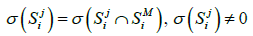 (2)
(2)
then it can be said that the metagenome spectrum covers the spectrum of genome j for primer i. It follows, obviously, that the necessary condition for a genome to belong to the metagenome is covering, for any primer, the genome spectrum by that of the metagenome. Below, this condition will be crucial for the validation of belonging a certain genome to the metagenome. It is obvious that such necessary condition will always have a one-sided error - the erroneous recognition of certain genomes as belonging to the metagenome. However, this error can be reduced by conducting a number of tests with different primers. In what follow, we study this possibility of such reduction-first, by computer simulation and then on the basis of a theoretical model.
Testing the presence of a certain bacterium in the metagenome
Bacterial genomes and primers: We use set B of 100 bacterial genomes described by us previously [23], Supporting Information). This set is sufficiently representative to provide the basic (typical) parameter values and demonstrate the algorithm behavior when used in actual calculations.
The primers are generated randomly, with equal probability of occupying each primer position by nucleotides A, T, C, or G. The set of 100 primers obtained in this way is denoted as P.
In this study, the range of 50-1000 is chosen for the positions of spectral bands. Indeed, in 2.5 % agarose gel, the range of recognizable fragment lengths is just from 50 ôþ 1000 [24]; thus the number of spectral band positions n=950. We assume that the genome spectra for each primer from set P should have a relatively small number of bands. Since it is impossible to fix this number accurately, the above assumption will be referred to the average number of bands in a spectrum over all the genomes from set B. In this paper, two groups of primers will be considered, namely, those with the average number of spectral bands over all the tested genomes equal to 10 or 30. Thus, for a random set of 100 primers of length 7, without errors, the average number of bands in the spectrum of all the bacteria which belong to set B is equal to 9.55≈10 over the whole set of the primers considered, the average number of fragments being 10.3. For a random set of 100 primer of length 11, with two errors, the average number of bands is equal to 29.57≈30, the average number of fragments being 34.6. Denote the above two primer sets as P10 and P30.
Now consider metagenomes of size 10 or 50. Size 10 models the analysis peculiarities for metagenomes consisting of a small number of genomes, while size 50 models relatively large metagenomes.
Computer simulation: To test the algorithm, metagenomes of the two selected sizes (10 and 50 genomes) were constructed by randomly (with equal probability) choosing the required number of genomes from the 100 genomes of set B. Regardless of the metagenome choice, sets of primers of sizes 5 or 12 were also randomly selected from the 100 available primers of sets P10 or P30. For each genome of the bacterium not belonging to the metagenome under consideration and for each selected primer, it was determined whether the spectrum of this genome was covered by the metagenome spectrum. Then, in a random order, series consisting of 1, 2, ... , 5 primers and a separate series of 12 primers were used. Obviously, with the increase of the number of primers used (the length of the series), the number of the bacterial genomes that are not covered by the metagenome spectrum at least once, generally speaking, decreases. This number gives the error percentage. The described procedure was repeated 1,000 times. The precision of the method was evaluated based on the total fraction of errors. The error probabilities decrease exponentially with the increase of the primer numbers from 1 to 5. Indeed, for a metagenome consisting of 10 genomes (Table 1), the number of erroneously detected genomes decreases as ~0.59s , 1 ≤ s ≤ 5 where s is the number of primers from set P10 used in the testing procedure. For a metagenome consisting of 50 genomes, the number of erroneously detected genomes decreases as ~ 0.63s , 1 ≤ s ≤ 5. Similarly, for primer set P30, the error decreases as ~0.26s and as ~0.39s (1 ≤ s ≤ 5) in the case of the metagenome size 10 and 50, respectively.
| |S| | 10 | |||||||||||
|---|---|---|---|---|---|---|---|---|---|---|---|---|
| |M| | 10 | 50 | ||||||||||
| |p| | 1 | 2 | 3 | 4 | 5 | 12 | 1 | 2 | 3 | 4 | 5 | 12 |
| % (a) | 1.19 | 0.73 | 0.44 | 0.25 | 0.15 | 0 | 7.2 | 5.06 | 3 | 1.91 | 1.2 | 0.1 |
| % (b) | 1.8 | 0.72 | 0.36 | 0.16 | 0.07 | 9.63 | 4.37 | 2.4 | 1.29 | 0.73 | ||
| |S| | 30 | |||||||||||
| |M| | 10 | 50 | ||||||||||
| |p| | 1 | 2 | 3 | 4 | 5 | 12 | 1 | 2 | 3 | 4 | 5 | 12 |
| % (a) | 2.26 | 0.51 | 0.15 | 0.04 | 0.01 | 0 | 18.28 | 6.36 | 2.2 | 0.96 | 0.4 | 0.4 |
| % (b) | 2.28 | 0.53 | 0.17 | 0.06 | 0.03 | 18.02 | 7.97 | 4 | 2.15 | 1.35 | ||
Table 1: Percentage of errors for different parameters of the metagenome and of the primers. Rows: primer weight, |S|; metagenome size, |M|; the number of primers in a series, |p|. Calculations were performed using (a) simulation or (b) the model (see Comparison of computer-simulation and model-based results).
Computer-simulation using a natural metagenome: In this section we perform a similar simulation using a natural metagenome, that is, the one that comprises a natural combination of bacteria. We use the data on the composition gut metagenomes, [25], 90% of which consists of the following ten bacteria: Akkermansia muciniphila ATCC BAA-835, Alistipes shahii WAL 8301, Bacteroides vulgatus ATCC 8482, Bifidobacterium adolescentis ATCC 15703, Coprococcus sp. ART55/1, Eubacterium eligens ATCC 27750, Faecalibacterium prausnitzii L2-6, Lachnospiraceae bacterium 1 4 56FAA, Prevotella copri DSM 18205 and Ruminococcus sp. 18P13. The corresponding genomes (some of them in the draft form) were found on the NCBI site. Naturally, in an actual investigation, the rest of 10% genomes will also appear important, but in this study we confine ourselves to the above 10 genomes since they represent a natural combination, which is just our aim.
The metagenome was modeled by a mixture of randomly chosen nine genomes from the ten ones listed above. To estimate the probability of not belonging the tenth genome to the metagenome, simulation was performed using random markers from set P10. The number of simulations was 1000. When five or 12 markers were used, the percent of erroneous results was 0.2 and 0%, respectively.
Theoretical model for estimating the genome inclusion in the metagenome and comparing it with the results of computer simulation
Previously in connection with the evaluation of the number of DNA fragments in one band, the occupancy model was used [26,27]. In the present study, we use this model to estimate the probability of the coincidence of the spectral bands for the genomes constituting the metagenome, i.e., to the estimation of the number of bands in the metagenome spectrum. In this model, the distribution of the spectral bands of all the above genomes by boxes should simulate the probability of their coincidence.
The distribution of lengths of genome fragments in the marker analysis is non-uniform, short fragments prevailing [26,28]. The distributions of the bands across all the genomes of set B and across all the primers from sets P10 and P30, obtained by the simulation procedure described in Computer simulation of metagenome analysis, are shown in (Figures 1A and B). Although the empirical distributions of the band frequencies obtained by us contain much more noise than the genome fragment distributions obtained in silico [26], the form and the widths of the distribution curves are in good agreement.

Figure 1: Frequency distribution of the band lengths of the genomes from set B (A) for primer set P10; (B) for primer set P30. Abscissa axis: the band length (from 50 to 1000). Frequency distribution of the boxes in the occupancy model (C) for primer set P10; (D) for primer set P30. Abscissa axis: the order of the boxes (from 1 to 950), which is different for different graphs.
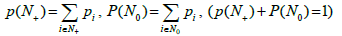
The probability distributions (Figures 1C and D) of occurring a band in the box is obtained from the band distributions (Figures 1A and B) by ordering the boxes in the order of descending probability. Denote the probability of the band to occur in the i-th box by pi , Σpi =1 Since the probability distributions are not uniform, the generalized version of the occupancy problem should be used, where the probabilities of filling the boxes are not supposed to be equal [29].
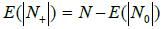
Filling the boxes leads to the partition of the entire box set into two subsets: those containing no bands (N0) and those containing at least one band (N+) fragment. For each particular filling, the sums define the probability (measure) of the corresponding sub-sets. If the tested genome has ν fragments, it can be assumed that the probability of covering its spectrum by the metagenome one is p(N+)ѵ (provided that the genome does not belong to the metagenome). Thus, in our case, the value of p(N+) is the crucial parameter of the occupancy model.
In our case, the drawback of the model is that the occurrences of the bands in a particular box are independent of each other. However, the formulation of the problem implies that the bands belonging to the same genome cannot occur in the same box, even two of them. Let us estimate the error of occurring more than one band of the same genome in the same box. Expectation  of the number of free boxes is [29]
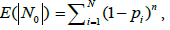 (3)
(3)
where n is the number of elements (in our case, bands) distributed into boxes. Consequently, the value of
 (4)
(4)
is the average number of boxes occupied by at least one band. Let us introduce matrix GP (100×100), each element of it being the number of bands for the corresponding bacteria-primer pair (i.e., the value of n). Using this matrix and the probability distributions presented in Figures 1C and D for each such pair, calculate the number of occupied boxes, using formula (4), and then average the numbers over all the pairs. As a result, for the primers of sets P10 and P30, the average number of occupied boxes is 9.98 and 30.22, respectively. This means that, on average, 10 or 30 boxes will be occupied, which is equal to the average number of bands in the genome of each series. Consequently, occurring of two bands of the same genome in one box is a rare event and will not have significant effect on the result. Of course, this is true for a relatively small number of bands in the genome spectrum, but even for the number of bands being 50, according to (4), on average, only one pair of bands can occur in the same box for a given probability distribution and only five bands overlap in different ways with for a spectrum of 100 bands.
Estimation of the total probability of the set of free and occupied boxes
In the case of the uniform occupancy problem, i.e., when  i = 1,...,N, the expectancy for the number of free boxes is
  [29]. Consequently, the probability measure of such set is
 In the case of unequal probabilities, there exists an exact formula for the expectation of the probability measure, which, in its original form, is the total enumeration formula over all the subsets of set N and, obviously, cannot be used for sufficiently large values of N. Below we consider the expectation of the probability measure, provided that the subset of free boxes is of fixed size. However, since even in this case, the initial formula is also of little use for direct calculations, we will confine ourselves by the quadratic approximation of the mathematical expectation.
If the pre-set number of free boxes is ν, then in the uniform model, the corresponding expectation is, obviously, ѵ/ N, and, as a result, the probability measure expectation for the set of occupied boxes is (N- ѵ)/N, which is the zero approximation. In the general case, the probability of set of boxes {i1, i2 , … , iv ) (and only of this set) being uncovered when n objects are distributed in N boxes equals
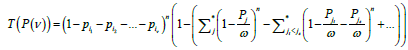 (5)
(5)
where * in the summation sign denotes summation over all the subsets of set P/P(ѵ) and the value of ω is equal to the sum of all probabilities of the same set: 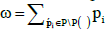 . Factor
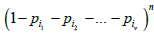 in (5) is the probability of all the boxes from set P(ѵ) being empty. The second factor in (5) is the probability of all the boxes from set P/P(ѵ), complementary to P(ѵ), being occupied.
Thus, the value of T(P(ѵ)) is equal to the probability of exactly ν boxes of set P(ѵ) remaining empty for n trials. Then expression
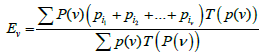 (6)
(6)
is the expectation of the total probability of all the sets of ν-sized boxes that may remain empty. (The summation is performed over all subsets composed of ν boxes.)
Statement: The asymptotic expression for the mathematical expectation of the probability measure value for empty and occupied boxes is
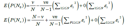 (7)
(7)
The value of n is the total number of spectral bands for the genomes constituting a metagenome, N is the number of different possible band lengths,  and ν is the pre-set value of empty boxes. The evaluation of (7) is given in Appendix.
Comparison of computer-simulation and model-based results
Since the probability distributions in Figure 1 differ little from the uniform one, one approximation (7) can be applied to the former data. In the framework of this approximation, we choose the volume, ν, of the empty boxes set equal to this volume expectation, which can be effectively computed by (3) for a given number of bands in the metagenome. Assume that the volume of the set to be distributed equals to n= |M| σ(p*) where |M| is the number of different genomes in the metagenome and σ(P*), is the average number of bands per one genome for primer sets P10 or P30. Then three expectation estimates E(P(N+)) of the probability measure of the occupied boxes set are obtained (Table 2): (1) the mean over 10000 of simulated distributions into the boxes; (2) the mean over the simulated distributions under condition of the empty set volume being equal to the mathematical expectation of the empty boxes volume; (3) with calculations performed using (7).
| 10 | 50 | |||||
|---|---|---|---|---|---|---|
| a | b | c | a | b | c | |
| 10 | 0.102 | 0.101 | 0.102 | 0.414 | 0.414 | 0.415 |
| 30 | 0.283 | 0.283 | 0.284 | 0.796 | 0.796 | 0.802 |
Table 2: The mean total probabilities, E(P(N+)) of boxes sets occupied by the metagenome bands. Row 1: the number of different genomes in the metagenome. Column 1: The mean value of bands in the genomes for the primers from sets P10 and P30. (a) Results obtained by computer simulation of the boxes occupation by the metagenome bands. (b) The same under condition of N-ν boxes being occupied, where N-ν is the mean number of boxes occupied in case (a). (c) Results obtained on the basis of (7), which are, actually, the approximation of the values in (b).
Next, using matrix GP, we calculate probability ω PG(i, j) of occurring all the i-th genome bands, for primer j, in the boxes already occupied by the metagenome bands, where GP(i,j) is the number of the bands and ω is the total probability of occupied boxes for all sets of parameters (Table 2). The mean values of the calculated probabilities (mean errors of testing) for different metagenome sizes are presented in Table 3.
| 10 | 50 | |||||||
|---|---|---|---|---|---|---|---|---|
| a | b | c | d | a | b | c | d | |
| 10 | 1.80 | 1.78 | 1.80 | 1.19 | 9.60 | 9.60 | 9.63 | 7.20 |
| 30 | 2.20 | 2.21 | 2.28 | 2.26 | 17.15 | 17.09 | 18.02 | 18.28 |
Table 3: Average percentage of errors in testing genomes for different metagenome sizes. (a)-(c) the same as in Table 2, (d) results of computer simulation by RAPD using natural genomes (Table 1).
In Table 3, the average probabilities are converted to percentages in order to facilitate the comparison with the results obtained by RAPD simulation, which proved to be in good agreement with the model-based results (Table 1).
The error percentages with primer series were calculated in the following way. For each genome i, primer jm from the selected primer series, which gave the largest number of bands, was determined using matrix GP. It was this number of GP (I,jm) that was used for calculating probability ωGP(i, jm ) of occurring the genome spectrum in the boxes set occupied by the metagenome bands.
The model-based calculation results are presented in Table 1. It can be seen that they are in good agreement with the computersimulation results also shown in Table 1.
Finally, let us use the model to calculate the possibility of comparing the tested genome with a metagenome composed of 100 genomes. For primer set P10,, the estimate value of  is 0.65, which gives the error of 21.1% for one primer. For primer set P30, the value of is
  1.00, which means that such a metagenome cannot be examined because it covers any genome.
The proposed model of distribution over boxes is, actually, fundamental in the random distribution processes for objects of various types. It is applicable for the particles in Boltzmann statistics modeling as well as for the distribution of DNA fragments over their lengths. The calculations to be performed in this model are rather complicated. Indeed, in expression (5) the summation is done over all the subsets of fixed length belonging to a certain set. The number of such subsets can grow exponentially: for example, at ν=N/2 it grows as 2N. Thus direct calculations according to formulae (5) become ineffective already at relatively small values of N (~100). The asymptotic technique proposed in this work is one of possible ways to make the calculations feasible.
Conclusion
On the basis of the results presented above, a simple twostep method of testing a metagenome can be proposed. First, the spectrum of the metagenome under consideration is determined for a certain number of primers, the amount of which should be small (according to our results of computer modelling). The time of this in vitro assessment does not depend on the number of primers since the corresponding spectra can be recorded simultaneously. Second, the metagenome spectra are compared with the spectra of the genomes being searched for, which are already known and collected in genome spectra libraries. This step is also performed quite fast. As described above, if a genome spectra obtained for 5 primers are covered by the corresponding metagenome spectra, it can be concluded that the genome is present in the metagenome, the error being 1%.
The composition of the metagenome is not limited in any way; in particular, it may contain unknown genomes. In most of the examples discussed above, the number of different genomes in the metagenome was limited to 50 because the number of possible spectral band positions WA only 1,000. Since the same mixture of fragments can be separated on gels of various concentrations, the number of the spectral bands can be increased from 50 to 15,000 [24]. Thus a bacterial metagenome composed of up to 3,000 different genomes can be examined. Using such a large number of bands makes it possible to study bacterial metagenomes in the presence of human DNA (it was shown by computer simulation in the equiprobable band-lengths approximation [23].
The proposed method allows detecting the genome to be tested in a broad range of microorganisms, including bacteria, fungi, and protozoa. The alternative methods to the one proposed in this work essentially imply DNA sequencing - either after cutting a specific gene out of the genome or sequencing the whole genome. In any case, sequencing is still more expensive and time-consuming than the marker method.
However, there exists a situation, in which additional sequencing is still required after using the proposed method. It is often necessary to identify also the microorganism strain. Different strains of the same microorganism usually originate from minor variations in certain genes, which do not cause any differences in the spectra. In such cases, one of the standard methods of strain identification should be used. For example, there exist special PCR primers for “cutting out” the genome fragments where the variation is localized. These fragments are sequenced and thus the gene allele is established. The primers under consideration are known for all microorganisms that have virulent strains. However, these primers are quite different for different microorganisms, which make the possibility of fast preliminary identifying the microorganism (bacterium) type by the method proposed in our manuscript especially important.
The algorithm proposed in this work can be used with the DNAmarker method of any type (Appendix).
References
- Doyle CJ, O'Toole PW, Cotter PD (2017) Metagenome -based surveillance and diagnostic approaches to studying the microbial ecology of food production and processing environments. Environ Microbiol 19: 4382-4391
- Katz M, Hover BM, Brady SF (2016) Culture-independent discovery of natural products from soil metagenomes. J Ind Microbiol Biotechnol 43: 129-141.
- Tkacz A, Poole P (2015) Role of root microbiota in plant productivity. J Exp Bot 66: 2167-2175
- Bulgarelli D, Schlaeppi K, Spaepen S, Themaat EVL, Schulze-Lefert P (2013) Structure and functions of the bacterial microbiota of plants. Annu Rev Plant Biol 64: 807-838
- Bhattacharyya PN, Tanti B, Barman P, Jha DK (2014) Culture-independent metagenomics approach to characterize the surface and subsurface soil bacterial community in the Brahmaputra valley, Assam, North-East India, an Indo-Burma mega-biodiversity hotspot. World J Microbiol Biotechnol 30: 519-528.
- Dorn-In S, Bassitta R, Schwaiger K, Bauer J, Hölzel CS (2015) Specific amplification of bacterial DNA by optimized so-called universal bacterial primers in samples rich of plant DNA. J MicrobiolMethods 113: 50
- Teranishi H, Ohzono N, Inamura N, Kato A, Wakabayashi T, et al. (2015) Detection of bacteria and fungi in blood of patients with febrile neutropenia by real-time PCR with universal primers and probes.J Infect Chemother 21: 189-193
- Takahashi S, Tomita J, Nishioka K, Hisada T, Nishijima M (2014) Development of a prokaryotic universal primer for simultaneous analysis of Bacteria and Archaea using next-generation sequencing. PLoS One 9: e105592.
- Lu JJ, Perng CL, Lee SY, Wan CC (2000) Use of PCR with universal primers and restriction endonuclease digestions for detection and identification of common bacterial pathogens in cerebrospinal fluid. J Clin Microbiol 38: 2076-2080.
- Ullberg M, Lüthje P, Mölling P, Strålin K, Ozenci V (2017) Broad-Range Detection of Microorganisms Directly from Bronchoalveolar Lavage Specimens by PCR/Electrospray Ionization-Mass Spectrometry. PLoS One 12: e0170033
- French K, Evans J, Tanner H, Gossain S, Hussain A (2016) The Clinical Impact of Rapid, Direct MALDI-ToF Identification of Bacteria from Positive Blood Cultures. PLoS One 11: e0169332
- Kok J, Thomas LC, Olma T, Chen SCA, Iredell JR (2011) Identification of bacteria in blood culture broths using matrix-assisted laser desorption-ionization Sepsityper™ and time of flight mass spectrometry. PLoS One 6: e23285.
- Rödel J, Bohnert JA, Stoll S, Wassill L, Edel B, et al. (2017) Evaluation of loop-mediated isothermal amplification for the rapid identification of bacteria and resistance determinants in positive blood cultures. Eur J Clin Microbiol Infect Dis 36: 1033-1040.
- Fidler G, Kocsube S, Leiter E, Biro S, Paholcsek M (2016) DNA Barcoding Coupled with High Resolution Melting Analysis Enables Rapid and Accurate Distinction of Aspergillus species. MedMycol 55: 642-659.
- Bertelli C, Greub G (2013) Rapid bacterial genome sequencing: methods and applications in clinical Microbiology. Clin Microbiol Infect 19: 803-813.
- Christensen JE, Stencil JA, Reed KD (2003) Rapid Identification of Bacteria from Positive Blood Cultures by Terminal Restriction Fragment Length Polymorphism Profile Analysis of the 16S rRNA Gene. J Clin Microbiol 41: 3790-3800
- Pallen MJ, Loman NJ, Penn CW (2010) 0High-throughput sequencing and clinical microbiology: progress, opportunities and challenges. Curr Opin Microbiol 13: 625-631.
- Williams JG, Kubelik AR, Livak KJJ, Rafalski A, Tingey SV (1990) DNA polymorphisms amplified by arbitrary primers are useful as genetic markers. Nucleic Acids Res 18: 6531-6535.
- Mueller UG, Wolfenbarger LL ( 1999) AFLP genotyping and fingerprinting. Trends Ecol Evol (Amst.) 14: 389-394.
- Vos P, Hogers R, Bleeker M, Reijans M, van de Lee T, et al. (1995) AFLP: a new technique for DNA fingerprinting. Nucleic Acids Res 23: 4407-4414.
- Saiki RK, Scharf S, Faloona F, Mullis KB, Erlich HA, et al. (1985) Enzymatic amplification of beta-globin genomic sequences and restriction site analysis for diagnosis of sickle cell anemia. Science 230: 1350-1354.
- Kirzhner V, Volkovich Z (2016) Analysis of Metagenome Composition by the Method of Random Primers. Eprint arXiv.
- Kirzhner V, Volkovich Z (2012) Evaluation of the Genome Mixture Contents by Means of the Compositional Spectra Method. Eprint arXiv
- Sambrook J, Fritsch EF, Maniatis T (1989) Gel electrophoresis of DNA. In: Sambrook J, Fritsch EF, Maniatis T (eds) Molecular Cloning: a Laboratory Manua, New York: Cold Spring Harbor Laboratory Press, Cold Spring Harbor, NY, USA.
- Dubinkina V, Ischenko D, Ulyantsev V, Tyakht A, Alexeev D (2016) Assessment of k-mer spectrum applicability for metagenomic dissimilarity analysis. BMC Bioinformatics 464: 7285.
- Gort G, Koopman WJM, Stein A (2006) Fragment Length Distributions and Collision Probabilities for AFLP Markers. Biometrics 62: 1107-1115.
- Feller W (1971) An Introduction to Probability Theory and Its Applications. Vol 1 (2nd edtn), John Wiley.
- Gort G, Koopman WJM, Stein A, Van Eeuwijk FA (2008) Collision Probabilities for AFLP Bands, with an Application to Simple Measures of Genetic Similarity. J Agri Biol Environ Stat 13: 177-198
- Kolchin VF, Chistiakov VP, Sevastianov BA (1978) Random Allocations, Washington: VH Winston, New York.