Research Article, J Electr Eng Electron Technol Vol: 6 Issue: 1

Time-Domain Methodology for the Relatively Low-Frequency Characterization of Large Antennas

Rammal R¹, Hejase HAN^2* and Assi A¹

¹Department of Electrical and Electronic Engineering, Lebanese International University, Beirut, Lebanon

²Faculty of Applied Sciences, American University of Technology, Fidar-Halat, Lebanon

*Corresponding Author : Hassan A.N. Hejase
Faculty of Applied Sciences, American University of Technology, Fidar-Halat, Lebanon
Tel: +961-78-819263
E-mail: hhejase@ieee.org

Received: April 24, 2017 Accepted: May 10, 2017 Published: May 17, 2017

Citation: Rammal R, Hejase HAN, Assi A (2017) Time-Domain Methodology for the Relatively Low-Frequency Characterization of Large Antennas. J Electr Eng Electron Technol 6:1. doi: 10.4172/2325-9833.1000138

Abstract

Keywords: Outdoor measurement; Time-domain acquisition; Cylindrical; Nearfield to far-field transformation; Antenna characterization

Introduction

Time-domain antenna measurements allow for antenna characterization in an ordinary laboratory or outdoor environment and eliminate the need for expensive anechoic chambers and their costly maintenance. Time-domain data acquisition allows the evaluation of frequency-domain values in the bandwidth covered by the excitation signal, and significantly reduces the measurement time needed, especially for the characterization of wideband antennas, since data acquisition is made only once. This methodology can be easily adapted for small and relatively large directive structures and allows for the characterization of systems with multiple sources working at the same time with different frequencies. The novelty of this work resides in the association of outdoor time-domain measurement techniques to the well-known near-field (NF) to farfield (FF) transformations and proposes a measurement approach where other measurement techniques fail to present competitive solutions.

For electrically large antennas, such as base station and satellite communication antennas, the far-field region is assumed to hold if the minimum distance between the antenna probe and the antenna under test is larger than max (2D²/λ_max, 10λ_max). D denotes the largest antenna physical dimension, and λ_max is the maximum wavelength of measurement bandwidth. For such antennas, use of the anechoic chamber for far-field measurements becomes impractical due to the large dimensions involved. The same applies for physically large antennas in the low-frequency range (30 MHz−1 GHz). There will be no reflections in the time window if the time duration (T) is chosen to be less than 6 λ_max/c where c is the speed of light (c ≈3×10⁸ m/s).

Time-domain measurement techniques offer solutions for cases that are usually considered as limitations in antenna measurements. This approach employs a combination of near-field measurements and Fast-Fourier Transform (FFT) technique to generate the far-field patterns. The challenge resides in the selection of the appropriate sampling criteria that will help minimize the truncation error resulting from the FFT implementation.

Time-domain metrology consists of radiating an extremely limited time signal covering a predefined bandwidth [1]. The emitted signal is directly measured in the time-domain using a probe and a digital oscilloscope and applying time gating (windowing) to eliminate reflections from the surroundings. The radiated signal vanishes quickly and does not disturb the surrounding electromagnetic environment [2-5]. The time-domain metrology has been applied previously to characterize the transfer function of vegetation [6] and for multifilar connector characterization [7]. This principle is updated and implemented to measure antenna response, and its utility is proven when measuring antennas independently from their geometrical structures while placed in their real radiation environment in a complete electronic system. One convenient application is for vehiclemounted antennas [8]. On the other hand, far-field measurements require a high peak radiated power and can cause problems when eliminating echoes. Also, mounting and installation difficulties may appear when characterizing large radiating structures.

The problem of determining the antenna FF pattern from NF measurements has attracted considerable attention in the last few decades [9-26]. Bucci and Gennarelli [15] applied a sampling approach to reconstruct the antenna FF pattern from NF measurements on a cylinder. Ovidio et al. [24] presented an overview of the application of band-limitation properties and non-redundant sampling representations of electromagnetic fields to NF-FF transformation techniques. They introduced formulas for the efficient reconstruction of the NF data needed by the classical NF-FF transformation corresponding to the adopted scanning surface from the acquired non-redundant samples. D’Agostino et al. [25] have experimentally assessed a direct NF-FF transformation technique with cylindrical scanning, and which requires a minimum number of near-field data. Their method allows accurate reconstruction of the antenna’s FF pattern in any plane directly from the non-redundantly acquired near-field data, without the need for interpolation. Their approach yields a remarkable reduction in measurement time and eliminates the characteristic ripple caused by the discontinuity of the near field at the edge of the scanning area.

Levitas et al. [26] proposed an ultra-wide-band (UWB) system for time-domain NF antenna measurements with new time-domain data pre-processing algorithms and optically-fed antenna probe. The developed system is suitable for planar, cylindrical, and spherical NF antenna measurements. Their results are in good agreement with standard FF antenna measurements for the frequency range of 1–20 GHz. In an earlier work, Rammal et al. [23] used simulation and experimental results to validate the NF-FF FFT transformation algorithm for an UWB antenna.

This paper applies a time-domain measurement technique for antenna characterization. The procedure starts with NF time-domain data acquisition, followed by the NF to FF transformation algorithm to construct the FF radiation patterns and antenna gain. The near-field measurements are done using a field probe which is properly placed in the test region. The presence of the probe causes field distortion and hence contributes to measurement errors. Thus the formulation of near-field to far-field transformation algorithms requires a proper probe correction. The validation phase of the measurement setup considers two different antenna types (UWB and Narrow Band) with the narrow-band 'sectoral' antenna posing a challenge for timedomain measurements.

Measurement Configuration

Figure 1 depicts the proposed measurement setup. It consists of a transient pulse generator that feeds the transmitting antenna (Antenna Under Test- AUT), and a transient field sensor as the receiving antenna which is connected, through a balun, to a digital oscilloscope. This system permits the measurement of near-field values at the required positions by generating an extremely narrow pulse which does not disturb the electromagnetic environment, and whose spectral content corresponds to a large frequency spectrum.

The Kentech-APG1 pulse generator [27] produces a Gaussian pulse with a peak voltage of 220 V and a rise time of 116 ps and covers the 30 MHz−4.5 GHz frequency spectrum (at -10 dB) as shown in Figure 2. The digital oscilloscope used is a Tektronix TDS 6804B model having four digital input channels with 8 GHz bandwidth, a rise time of 50 ps (10%- 90%) and a sampling rate of 20 G Samples/s. The generated electric field is measured using a PRODYN AD-80 probe [28] that represents an electric dipole with a ground plane. The probe has a bandwidth of 5.5 GHz, a rise time below 64 ps, and a maximum output voltage of ±1 kV. Figure 3 shows the transfer function representing the ratio of output voltage to the radiated electric field received from the time-domain probe in its E-plane; the inverse of which represents the antenna factor. The probe’s transfer function is considered because of the dependence of electric field values on the sensor’s inclination angle.

The antenna under test (AUT), shown in Figure 1, is mounted on a single-axis turntable controlled by a brushless motor with the help of a LabVIEW algorithm through an NI GPIB IEEE-488 interface bus via an optical fiber link. The turntable can carry up to 1000 kg of weight with a rotational accuracy of ± 0.5⁰. The LabVIEW algorithm allows the generation of a time-domain pulse for each angular position and then waits for the signal to be sampled by the digital oscilloscope before moving to the next position.

The near-field probe is moved vertically along the height of the cylindrical surface (z-direction). The cylindrical surface is mapped by rotating the AUT with the turntable and moving the probe in the vertical direction, thus generating a grid of field samples along the azimuth and z coordinates. This measurement setup is ideally useful for base-station type Personal Communications Service (PCS) antennas, i.e., antennas with omnidirectional radiation pattern in one plane and minimal upward or downward radiated energy. The field sensor is positioned at different heights for each complete turn by the automated turntable. The measurement time needed for an angular step of 3⁰ is about 15 minutes.

The experimental setup, described in Figure 1, is used to measure the time-domain electric field tangential to the cylindrical surface surrounding the AUT. The radius of the near-field cylinder (imaginary measurement surface) must be as small as possible to minimize the number of measurement points and should satisfy the near-field range requirement of the AUT out of the Rayleigh zone. Furthermore, the spacing between sampling points needed to perform the cylindrical NF-FF transformation must meet the following conditions [9,18]:

(1)

With “a” being the radius of the smallest cylinder enclosing the device under test. The first condition fixes the maximum height of each sample (Δz); the second sets the largest angular increment (Δφ). Note that the arc length separating adjacent sample points on the smallest cylinder enclosing the antenna is Δs ≈ a Δφ ≈ λ/2.

Time gating

Time gating allows the elimination of parasitic reflections coming from obstacles neighboring the AUT such as ground, walls and any other equipment or objects. This operation depends on the radiated signal shape; i.e. for UWB antennas where the radiated time-domain signal is extremely short with little dispersion. The clear time T_c denotes the time required for the arrival of the first reflection considered coming from the ground (Figure 4). For narrow-band antennas (long time-domain signals) as well as for ‘undefined’ types, a preliminary measurement is necessary for computing T_c, which defines the radiating signal duration. T_c is then used to calculate the height at which the antenna must be placed to avoid any interference between the useful signal and parasitical echoes. The clear time is computed from Figure 4 using

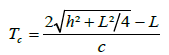(2)

where L is the distance between the AUT and the sensor, h is the height above ground, and c is the speed of light (≈3 × 10₈ m/s).

Far-field computation

The far-field pattern construction starts from the reflection-free time-domain tangential electric near field. The near-field to far-field transformation consists of two steps. The first step is to measure the values of E and H fields on a closed surface (Huygens’ surface) around the AUT, and then to seek secondary radiating sources using integral equations. The second step is to perform a modal expansion of the tangential near electric field, as a solution of the vector Helmholtz equation of propagation, which verifies the boundary conditions on the near-field measurement surface as well as at infinity [9-10,29]. The cylindrical coordinate system is chosen for the theoretical formulation of this transformation [9,15,23]. The coordinate system selection (rectangular, cylindrical, and spherical) depends on the geometry of the AUT [9] with the cylindrical coordinate system being more suitable for omnidirectional antennas, i.e., PCS antennas. The orthogonality properties of the modes on the cylindrical surface are then used to calculate the modal expansion coefficients thus allowing the reconstruction of the far-field pattern for the AUT.

The cylindrical near-field components and (N index for near-field) are directly computed from the measured time-domain tangential electric near fields on the Huygens’ cylindrical surface surrounding the antenna, using an FFT algorithm [9-15]. The spacing between measurement points must be arranged to make the aliasing error negligible. Equation (1) describes the standard sampling criteria adopted in cylindrical NF-FF transformation.

The spherical components of the far electric field (F index) are given by:

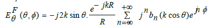(3)

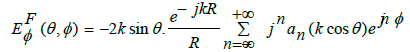(4)

Where a_n (k cosθ) and b_n (k cosθ) are modal coefficients which depend on two-dimensional spatial integrals of the measured harmonic near fields and [9-15,18,23]. These equations are programmed using MATLAB, and the developed algorithm uses the NF time-domain data to generate the FF radiation patterns in different planes for a chosen frequency.

Measurement Results and Discussion

The experimental testing and validation are performed for two types of antenna configurations (AUT), namely, UWB antenna (Scissor) and narrow-band antenna (Sectoral). Figure 1 depicts the used measurement setup.

The center of the AUT is placed 2.5 m above the turntable as per Figure 1. A preliminary measurement is done to predict the height of the NF measurement cylindrical surface (Huygens’ surface) for each of the two chosen antenna types in order to produce an equivalent to 20 dB reductions in field values with respect to the maximum. The electric field sensor is positioned vertically with a step size of Δz = 5 cm and with an azimuthal angular increment of Δφ= 3⁰, which is an oversampling when compared to the defined criteria. The oversampling is, however, still necessary for an initial validation. The turntable realizes a complete turn with a measurement time of 15 minutes. The total data acquisition time is about 15 (minutes) × 87 (vertical position) ≈ 22 hours for the Scissor antenna and 15 (minutes) × 47 (vertical position) ≈ 12 hours for the Sectoral antenna. The measurement time can be considerably reduced as will be shown later.

UWB “Scissor” antenna setup and results

The Scissor antenna [30,31] is a 60 × 100 cm UWB bifilar antenna (Figure 5) which is directive in both vertical (E) and horizontal (H) planes. Designed by XLIM Research Institute, the scissor radiates short pulses of high peak level (many kilovolts) with minimal distortion in the 300 MHz−2.5 GHz frequency band. Figure 6 illustrates the Scissor antenna gain spectrum.

The selected antenna allows the measurement of its global radiation on the NF cylindrical surface. Also, time-domain measurements using this antenna may be directly done in FF distances. The validation process concludes by comparing a constructed FF starting from NF time-domain measurements with the measured FF directly in FF distances. Figure 7 shows the flow chart for the validation steps.

Echoes elimination

The measured time-domain signal contains two components, namely the ‘useful’ signal and the unwanted parasitical reflections. The clear time T_c calculated from Equation (2) for this measurement setup is 3.7 ns. Figure 8 shows the time gating of a selected time signal with the sensor positioned at the nearest point to ground.

Scissor antenna measurement results and validation

Computation of the harmonic field components follows the elimination of the pulsed signal echoes. For the selected frequency, a Fourier Transform (FT) algorithm keeps one complex value from each transmitted time signal, corresponding to the selected frequency, and thus, the near field emitted from the AUT is computed at the cylindrical surface. Figure 9 shows the tangential electric NF (E_z) values at 1 GHz on this surface. These field values are used by the NF-FF transformation algorithm to construct the FF patterns in the vertical (E) and horizontal (H) planes.

On the other hand, FF time-domain measurements are done directly in E and H planes. Figures 10 and 11 illustrate shape and magnitude comparison between the measured FF values and those constructed using the NF-FF transformation.

In the vertical plane (E-plane), the theta range of the constructed values is 23° to 157° because of the limitation in the cylinder’s height (Figure 10). In the H-plane, the difference in shapes for the azimuthal range |φ| > 100° (Figure 11) is due to inconvenient installation configuration corresponding to these angles (the antenna set-up system).

Narrow-band “Sectoral” antenna

The “Sectoral” M-EBG (Metallic – Electromagnetic Band Gap) antenna (Figure 12), realized by the XLIM Research Institute, is a narrow-band antenna used to achieve the broadcast type of coverage required for wireless applications, especially in mobile communications [32]. It works in vertical polarization for uplink UMTS (Universal Mobile Telecommunication System), with a directivity of 18.5 dB at 1.95 GHz and a radiation beam width of at least 60º in the horizontal plane.

This antenna measures 16.4 × 120 cm and is fed through three square patches with 65 mm side, printed on a thin substrate layer (2 mm thickness, dielectric constant ε_r = 1.1) as seen in Figure 12. The M-EBG structure is placed at 8 cm over the ground plane, which is about λ/2 at its operating frequency of approximately 1.95 GHz.

Radiated time signal length

Narrow-band antennas spread their time signals with respect to time. Therefore, the clear time (T_c) is used to calculate the height at which the antenna must be placed to avoid any interference between the useful signal and parasitical echoes. A preliminary measurement evaluates the duration of the radiated time-domain signal by this antenna at 14 ns as seen in Figure 13, and which is later used as the needed clear time. The installation height is then found to be approximately 2.5 m. The Sectoral M-EBG antenna is fed by the pulse generator (APG1) via a 4-way power splitter. Figure 14 shows the validation steps.

Sectoral antenna measurement results and validation

The harmonic electric NF components were computed at 1.95 GHz (the antenna’s maximal gain frequency) following the removal of parasitic echoes. Figure 15 shows the contour plot of the E_z – component on the cylindrical NF surface. The measured near-field data are used by the NF-FF transformation algorithm to construct the FF patterns in the vertical (E) and horizontal (H) planes.

On the other hand, this antenna’s FF cannot be measured directly at FF distances because of its long-duration radiated time signal. Therefore, to validate this measurement bench for narrow-band antennas, the antenna’s gain is calculated by introducing the constructed FF values into the Friis transmission equation. Then, the results are validated by comparison with the gain measured using SATIMO’s Stargate measurement system [33]. Figures 16 and 17 show the validation of results for the E and H planes, respectively, with good agreement (within 0.8 dB for the main lobe). The disagreement in the sidelobes is due to the NF cylinder height (setup measurement limitation). A larger cylindrical surface height may be required to enhance the FF pattern away from the major lobe. The cost would be a longer measurement time resulting from the more substantial amount of required samples.

The setup instrumentation used limits measurements to the frequency band 80 MHz−4.5 GHz. However, the frequency band can be easily extended using measurement equipment with better frequency capabilities. The digital oscilloscope used (single-shot) has a dynamic range of -70 dB (100 MHz) to -30 dB (3 GHz), which is considered as a limitation when comparing to harmonic measurements whose dynamic range decreases from -20 dB (100 MHz) to -50 dB (3 GHz).

The data acquisition for each complete azimuthal turn using an angular step of 3° is about 15 minutes which is an extra sampling step. The measurement time can be reduced using the appropriate angular and vertical steps. Furthermore, automation of the acquisition and vertical positioning system can assure a notable reduction in measurement time.

The choice of antennas is limited to two extreme radiation types ranging from extremely narrow to extended time-domain radiated signals. Once validated, this measurement bench can be useful for the characterization of large antennas and complex radiation structures in the proposed frequency range.

The accuracy of the results obtained from the comparison of measurement data with SATIMO (Stargate constructor accuracy of ±1dB) is sufficient to validate this measurement technique. Further studies will address the accuracy range evaluation.

Conclusion

The proposed measurement bench allows the construction of farfield patterns of antennas and radiating sources from a single timedomain outdoor acquisition. The method is validated using both ultra-wide band (UWB) and narrow-band antennas.

The NF-FF transformation technique obtains the radiation pattern of any radiating structure over a wide band of frequencies, from a single time-domain data acquisition in the NF followed by a mathematical calculation. The results show reasonable agreement with direct FF measurements in terms of the shape of constructed signals, as well as field and gain values. This proposed measurement technique provides a ‘potential’ advantage in term of measurement time and cost while remaining non-disruptive to the environment with pulses of extremely short durations.

References

1. Rammal R, Assi A (2013) On the Electromagnetic Radiations Measurement. In: Proceedings of the13th Mediterranean Microwave Symposium (MMS’2013), Beirut, Lebanon.
2. Rammal R, Lalande M, Martinod E, Feix N (2011) Far-field and gain calculation starting from near-field time-domain data acquisition. In: Proceedings of the 5th European Conference on Antennas and Propagation (EUCAP); Rome, Italy.
3. Rammal R, Lalande M, Martinod E, Feix N, Hajj M, et al (2010) Outdoor transient measurement base in cylindrical coordinates for antenna characterization. In: Proceedings of the IEEE Antennas and Propagation Society International Symposium (APSURSI), Toronto, Canada.
4. Rammal R, Lalande M, Martinod E, Feix N, Jouvet M, et al. Large antennas characterization: Far–Field reconstruction using outdoor transient measurements for narrow and wide band radiating sources. In: Proceedings of the 4th European Conference on Antennas and Propagation (EUCAP), Barcelona, Spain.
5. Rammal R, Lalande M, Martinod E, Feix N, Andrieu J, et al (2009) Outdoor transient Ultra-wideband measurement techniques for antenna characterizations and radiation patterns. In Proceedings of the 3rd European Conference on Antennas and Propagation (EUCAP),  Berlin, Germany.
6. Dubois C, Chauvet V, Mallepeyre V, Gallais F, Bertrand V, et al (2004) The UWB SAR system PULSAR: Applications and Improvements. Poster session presented at: Radar 2004, Toulouse, France.
7. Martinod E, Bertrand V, Lalande M, Reinex A, JeckoB (2002) Behavior of multifilar connectors in electromagnetic compatibility: a new experimental transient approach. IEEE Trans. On Electromagnetic Compatibility (EMC);
8. https://doi.org/10.1109/TEMC.2002.801754
9. Chauvet V, Lalande M, Feix N, Martinod E, Andrieu J ( 2005) Application of transient ultra wide band measurement to characterize the radiation pattern of automotive antennas. 11th International Symposium on Antenna Technology and Applied Electromagnetics (ANTEM 2005), Saint-Malo, France.
10. Leach Jr. WM, Paris D (1973) Probe compensated near-field measurements on a cylinder. IEEE Trans. Antennas and Propagat.
11. Johnson RC, Ecker HA, Hollis JS (1973) Determination of far-field antenna patterns from near-field measurements. Proceedings of the IEEE.
12. Appel-Hansen J, Dyson JD, Gillespie ES, Hickman TG (1982) Antenna measurements In: A. W. Rudge, K. Milne, A. D. Oliver, and P. Knight, Eds. The Handbook of Antenna Design. Peter Peregrinus Ltd, London, Uk.
13. Yaghjian AD (1986) An overview of near-field antenna measurements. IEEE Trans. Antennas and Propagat.
14. Gillespie ES (1988) Special Issue on near-field scanning techniques. IEEE Trans. Antennas and Propagat
15. Hald J, Hansen JE, Jensen F, Larsen FH (1988) Spherical Near-Field Antenna Measurements. Peter Peregrinus Ltd, London, UK.
16. Bucci OM, Gennarelli C (1988) Use of sampling expansions in near-field-far-field transformation: the cylindrical case. IEEE Trans. Antennas and Propagat.
17.  Evans GE (1990) Antenna Measurement Techniques. Artech House, Boston, Mass, USA.
18. Slater D (1991) Near-Field Antenna Measurements. Artech House, Boston, Mass, USA.
19. Bucci OM, Gennarelli C, Riccio G, Savaresse C (1998) NF – FF transformation with cylindrical scanning: an effective technique for elongated antennas. IEEE Trans. Antennas Propagat.
20. Gennarelli C, Riccio G, D’Agostino F, Ferrara F, Guerriero R (2004) Near-Field—Far-Field Transformation Techniques. vol. 1, CUES, Salerno, Italy.
21. Gennarelli C, Riccio G, D’Agostino F, Ferrara F, Guerriero R (2006) Near-Field—Far-Field Transformation Technique. vol. 2, CUES, Salerno, Italy.
22. Ferrara F, Gennarelli C, Guerriero R, Riccio G, Savaresse C (2006) Computation of antenna directivity from cylindrical near-field measurements. Microwave and optical technology letters
23. Francis MH, Wittmann RW (2008) Near-field scanning measurements: theory and practice. In: C. A. Balanis, editor. Modern Antenna Handbook. Chapter 19. Hoboken, NJ: John Wiley & Sons
24. Rammal R, Lalande M, Martinod E, Feix N, Jouvet M (2009) Far-Field Reconstruction from Transient Near-Field Measurement Using Cylindrical Modal Development. International Journal of Antennas and Propagat.
25. Bucci OM, Gennarelli C (2012) Application of Nonredundant Sampling Representations of Electromagnetic Fields to NF-FF Transformation Techniques. International Journal of Antennas and Propagation 14 pages.
26. D’Agostino F, Ferrara F, Gennarelli C, Gennarelli G, Guerriero R, et al. (2012) On the Direct Non-Redundant Near-Field-to-Far-Field Transformation in a Cylindrical Scanning Geometry. IEEE Antennas and Propagat. Magazine
27. Levitas B, Drozdov M, Naidionova I, Jefremov S, Malyshev S (2013) UWB System for Time-Domain Near-Field Antenna Measurement. In: Proceedings of the 43rd European Microwave Conference, Nuremberg, Germany.
28. http://www.kentech.co.uk/PDF/APG1_manual.pdf
29. http://prodyntech.com/ddotff.htm
30. Stratton JA (1941) Electromagnetic Theory. McGraw-Hill, New York.
31. Andrieu J, Beillard B, Imbs Y (2000) Wide Band Scissors Antenna. French patent 99 14940. November 1999; International patent FR 0002905.
32. Andrieu J, Nouvet S, Bertrand V, Beillard B, Jecko B (2005) Transient Characterization of a Novel Ultra-Wide Band Antenna: The Scissors Antenna. IEEE Trans. Antennas Propagat.
33. Hajj M, Rodes E, Serhal D, Monediere T, Jecko B (2008) Design of Sectoral Antennas Using a Metallic EBG Structure and Multiple Sources Feeding for Base Station Applications. International Journal of Antennas and Propagat 8: 1-7.
34. http://www.satimo.com/content/products/sg-24