Spanish
  Chinese
  Russian
  German
  French
  Japanese
  Portuguese
  Hindi
Hindi Research Article, Res J Econ Vol: 1 Issue: 2
Empirical Evidence on the Geometrical Properties of Structural Change Trajectories
Denis Stijepic*
Chair of Macroeconomics, Department of Economics, University of Hagen, Germany
*Corresponding Author : Denis Stijepic
Department of Macroeconomics, University of Hagen, Universitaetsstr 41, D-58084 Hagen, Germany
Tel: +4923319872640
E-mail: denis.stijepic@fernuni-hagen.de
Received: November 20, 2017 Accepted: December 15, 2017 Published: December 22, 2017
Citation: Stijepic D (2017) Empirical Evidence on the Geometrical Properties of Structural Change Trajectories. Res J Econ 1:2.
Abstract
We study the long-run labor reallocation dynamics in the three-sector framework relating to agriculture, manufacturing, and services. In particular, we depict the labor reallocation data provided by Maddison and World Bank on standard simplexes, study the geometrical properties of the implied vector field, and derive the geometrical properties of stylized labor reallocation trajectories. Moreover, we discuss how these properties can be explained by the standard structural change literature and used for structural change analysis and prediction.
Keywords: Structural change; Sectors; Labor; Reallocation; Long run; Dynamics; Trajectory; Simplex; Geometry; Vector
Introduction
Structural change is one of the most persistent phenomena of the long-run development process. We focus on the long-run labor reallocation dynamics in the three-sector framework relating to agriculture, manufacturing, and services, which is a major concept for analyzing structural change. For an overview of the structural change literature, see, for example, [1-5]. Recent papers modeling structural change in the three-sector framework are, for example, [6-13]. In contrast to the previous studies, for example, [5], we depict the empirical structural change data on simplexes. In particular, we exploit the fact that (a) the structural change in a country can be represented by a trajectory on a standard 2-simplex and (b) different trajectories representing the structural change in different countries can be depicted on one and the same simplex and compared to each other.
While this approach is not necessarily ‘efficient’ when it comes to the derivation of quantitative facts of structural change, it allows us to identify very easily the clusters of structural data points, monotony characteristics of structural dynamics, trajectory intersections, and trajectory self-intersections. In other words, our approach allows us to immediately identify the geometrical properties of the empirically observable vector fields and trajectory portraits representing the structural change dynamics of a group of countries. This information can be used to derive the properties of the dynamic systems generating these trajectories [12,14] and exploited for (a) prediction of structural change dynamics in developed and developing economies [10,11] and (b) comparison of standard models’ assumptions and results with empirical data [13-15].
In our paper, we explain the simplex approach briefly, depict the empirical data by using it, discuss the geometrical stylized facts that can be derived on the basis of this depiction, and review briefly the existing theoretical explanations and applications of these stylized facts.
The rest of the paper is set up as follows. The next section is devoted to the mathematical prerequisites related to the description of structural change via trajectories on standard simplexes. Then, we depict the empirical structural change data provided by [16] and the World Bank World Databank on simplexes. In the main part of our paper, we formulate the stylized facts and discuss (a) the empirical evidence related to them, (b) their theoretical explanations based on the previous theoretical literature, and (c) the structural change predictions that can be made on their basis by relying on the results of the previous literature. Concluding remarks are provided in the last section of our paper.
Mathematical prerequisites
In this section, we recapitulate some geometrical concepts for structural change analysis, as introduced by [10-12,14].
While there are different mathematical notational conventions, we choose the following notation for reasons of simplicity: small letters (e.g., x), bold small letters (e.g., x), capital letters (e.g., X), and Greek letters (e.g., α) denote scalars, vectors/points, sets, and angles, respectively. R (N) denotes the set of real (natural) numbers.
Definition 1: The sectors 1, 2, and 3 represent the primary (or agricultural) sector, the secondary (or manufacturing) sector, and the tertiary (or services) sector, respectively. y1c(t), y2c(t), and y3c(t) denote the employment in sector 1, 2, and 3 at time t ∈ D ⊂ R in country c ∈ C ⊂ N, respectively. yc(t) := y1c(t) + y2c(t) + y3c(t) is the aggregate employment at time t in country c. xic(t) := yic(t)/yc(t) is the employment share of sector i at time t in country c. The vector xc(t) := (x1c(t), x2c(t), x3c(t)) indicates the cross-sector labor allocation at time t in country c. The term ‘structural change over the period [a,b] in country c’ refers to the long-run dynamics of the labor allocation xc(t) (over the period [a,b]).
This definition implies (1)-(3).
 (1)
(1)
 (2)
(2)

Consider the Cartesian coordinate system (x1, x2, x3). We can identify any point in the three-dimensional real space (R3) with its Cartesian coordinates (x1, x2, x3). It is well known that S (cf. (3)) is a two-dimensional standard simplex (henceforth, 2-simplex), which is a triangle with the following Cartesian coordinates of its vertices.
(1, 0, 0) := v1 (0, 1, 0) := v2 (0, 0, 1) := v3 (4)
For an illustration, see Figure 1. Henceforth, we omit the coordinate axes, as depicted in the right panel of Figure 1.

Figure 1: The 2-simplex in the Cartesian coordinate system (x1, x2, x3) with and without coordinate axes.
According to (3), all the points (x1, x2, x3) that satisfy the conditions x1+x2+x3 =1 and ∀i ∈{1, 2, 3} 0 ≤ xi ≤ 1 are located on the 2-simplex S, i.e., on the triangle depicted in Figure 1.
Definition 1 and (1)-(3) imply that we can depict the labor allocation xc(t) and its dynamics (i.e., structural change) on the 2-simplex S. For doing so, we rely on the concept of the trajectory, which we define as follows.
Definition 2: Let t0, t1,…tm be a sequence of time points in D and xc(t0), xc(t1),…xc(tm) be the corresponding sequence of structures on S, where m ∈ N. Moreover, let ∀t ∈ {t0, t1,…tm-1}, Lc,t denote the line segment connecting xc(t) and xc(t+1). The structural trajectory Tc(t0,…tm) of county c ∈ C covering the time period t0-tm is defined by (5).
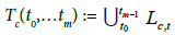 (5)
(5)
We indicate the direction of movement along the trajectory Tc(t0,…tm), i.e., the timely order of the points, by an arrow at the last observation point xc(tm).
Trajectories can be characterized by using the concepts of intersection, self-intersection, closeness (to the vertices of the simplex), and monotony. In our paper, we apply the following formal definitions of non-(self)-intersection.
Definition 3: The trajectory (5) is non-self-intersecting (for a given c ∈ C) if ∀t ∈ {t0, t1,…tm–1}, the line segments Lc,t constituting the trajectory (5) are pairwise disjoint, i.e.,
 (6)
(6)
Definition 4: Two trajectories Ta(t0,…tm) and Tb(t0,…tn), where a,b ∈ C and m,n ∈ N, intersect if 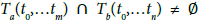 . Otherwise, if
 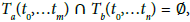 the trajectories Ta(t0,…tm) and Tb(t0,…tn) do not intersect.
For an example of a non-self-intersecting trajectory (selfintersecting trajectory), see, e.g., Figure 2a (Figure 2b). The trajectories in Figure 2c (2d) are intersecting (non-intersecting).

Figure 2: Examples of (non-)self-intersecting and (non-)intersecting trajectories on S.
Definition 5: A point xc(t) ≡ (x1c(t), x2c(t), x3c(t)) ∈ S is close to the vertex vi if and only if xic(t) > 0.5, where i ∈ {1,2,3}, c ∈ C, and t ∈ D.
Note that (3) and Definition 5 imply that a point can never be close to two or more vertices at the same time. A geometrical interpretation of Definition 5 is given by the following partitioning of the simplex S.
 (7a)
(7a)
S0 := S \ (S1 ∪ S2 ∪ S3) (7b)
Definition 5 and (7) imply the following statements [10,11]: a point is close to the vertex v1 if and only if it is located in the partition S1; a point is close to the vertex v2 (v3) if and only if it is located in the partition S2 (S3); a point is not close to any of the vertices if and only if it is located in the partition S0 (see also Figure 3).

Figure 3: A geometrical interpretation of Definition 5 and (7).
Definitions 1 and 5 imply the following economic interpretation of the notion of closeness to the vertices of S: if the labor allocation in country c is represented by a point close to the vertex vi, sector i employs more than 50% of the country c labor force, i.e., country c is dominated by sector i. For example, if the labor allocation at time t in country c is represented by a point (xc(t)) close to the vertex v3, country c is dominated by services at time t, i.e., x3c(t) > 0.5 > x2c(t) + x1c(t) (cf. (1)-(3)).
Definition 6: The vector angle αc(t) is the angle between the trajectory segment Lc,t and the simplex-edge v1v2 (cf. (4) and Figure 4), i.e., 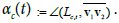

Figure 4: An example illustrating the vector angle αc.
Property 1 (cf. Definition 6). a) 120°<αc(t)<300° ⇒x1c(t+1)– x1c(t)> 0. b) 0°<αc(t)< 120° V 300°<αc(t)<360° ⇒x1c(t+1)–x1c(t)< 0. c) αc(t) ∈ {120°, 300°} ⇒ x1c(t+1)–x1c(t) = 0.
Property 2 (cf. Definition 6). a) 0°<αc(t)<60° V 240°<αc(t)<360° ⇒ x2c(t+1) –x2c(t)> 0. b) 60°<αc(t)<240° ⇒ x2c(t+1) –x2c(t)< 0. c) αc(t) ∈ {60°, 240°} ⇒ x2c(t+1) – x2c(t) = 0.
Property 3 (cf. Definition 6). a) 0°<αc(t)<180° ⇒ x3c(t+1) –x3c(t) > 0. b) 180°<αc(t)< 360° ⇒ x3c(t+1) –x3c(t)< 0. c) αc(t) ∈ {0°,180°} ⇒ x3c(t+1) – x3c(t) = 0.
For a detailed discussion of the economic interpretation of the (tangential) vector angles associated with labor allocation trajectories, see [10,11]. We can use Properties 1-3 to immediately identify the dynamics of the sectoral employment shares associated with a trajectory and, in particular, the trajectory segments characterized by monotonous dynamics of sectors. The following examples illustrate how Properties 1-3 can be used for analyzing trajectories.
Example 1: If each of the line segments Lc,t associated with the trajectory (5) is characterized by a vector angle between 0° and 120° or between 300° and 360°, then the employment share of the agricultural sector decreases monotonously along the trajectory (5), as stated by Property 1. See Figure 4 for an example of a trajectory depicting a monotonously decreasing agricultural share.
Example 2: Property 2 states that if each of the line segments Lc,t associated with the trajectory (5) is characterized by a vector angle of 60° or 240°, then the employment share of the manufacturing sector is constant along the trajectory (5). Thus, the employment share of the manufacturing sector is constant along the trajectory that is linear and parallel to the v3v1-edge of the 2-simplex.
Example 3: If each of the line segments Lc,t associated with the trajectory (5) is characterized by a vector angle between 0° and 180°, then the employment share of the services sector increases monotonously along the trajectory (5), as stated by Property 3. Figure 4 depicts a trajectory along which the services share increases (strictly) monotonously.
Structural change data presented on simplexes
Assume that we have data on the labor allocation (xc(t)) in country c for the time points t0, t1,…tm. According to Definition 2, we construct the labor allocation trajectory of country c by depicting the points xc(t0), xc(t1),…xc(tm) on the standard 2-simplex and connecting them by line segments (while preserving their timely order). We indicate the direction of movement along the trajectory (i.e., the timely order of the points) by an arrow at the last observation point. We do this procedure with all the countries for which we have data and depict the trajectories of all the countries belonging to a country group (e.g., OECD countries) on one simplex such that we can identify the intersections of the trajectories of the countries belonging to this group.
In Figures 5-7, we depict the data on the long-run labor allocation dynamics in the OECD countries (and Russia and China) on the 2-simplex, where the latter refers to the employment shares of agriculture (x1), manufacturing (x2), and services (x3) and the vertices (v1, v2, and v3) are given by (4). For better visibility, Figure 7 depicts the enlarged segment of Figure 6 containing all the trajectories depicted in Figure 6. In Figures 6 and 7, we omit the arrows indicating the direction of movement along the trajectories in the most cases for reasons of clarity. Furthermore, note that while Figure 5 depicts low-frequency data on structural change covering a very long period of time (i.e., 1820–1992), Figures 6 and 7 present high-frequency data on labor allocation dynamics over the period 1980–2015.

Figure 5: The labor allocation trajectories of USA, France, Germany, Netherlands, UK, Japan, China, and Russia.

Figure 6: The labor allocation trajectories of OECD countries over the 1980s, 1990s, 2000s, and 2010s.

Figure 7: The labor allocation trajectories depicted in Figure 6, enlarged.
Notes on Figure 5: Data source: [16]. The black dot represents the barycenter of the simplex. Abbreviations: C – China, F – France, G – Germany, J – Japan, N – Netherlands, R – Russia, US – United States, UK – United Kingdom. Data points (years in parentheses): USA (1820, 1870, 1913, 1950, 1992), France (1870, 1913, 1950, 1992), Germany (1870, 1913, 1950, 1992), Netherlands (1870, 1913, 1950, 1992), UK (1820, 1870, 1913, 1950, 1992), Japan (1913, 1950, 1992), China (1950, 1992), Russia (1950, 1992).
Notes on Figure 6: Data source: The World Bank, World Databank. The black dot represents the barycenter of the simplex. Arrows indicating the direction of movement along the trajectories are omitted in the most cases for reasons of clarity of representation.
Notes on Figure 7: The black dot represents the barycenter of the simplex. The edges of the simplex are not visible in Figure 7. Arrows indicating the direction of movement along the trajectories are omitted in the most cases for reasons of clarity of representation.
Figures 8-10 depict the data on less developed countries. Again, we distinguish between low-frequency data (cf. Figure 8) and higherfrequency data (cf. Figures 9 and 10). Figure 10 depicts the enlarged segment of Figure 9 containing all the trajectories depicted in Figure 9.

Figure 8: The labor allocation in 1950 and 1980 in emerging countries.

Figure 9: The labor allocation trajectories of non-OECD countries over the 1980s, 1990s, 2000s, and 2010s.

Figure 10: The labor allocation trajectories depicted in Figure 9, enlarged.
Notes on Figure 8: Data source: [16]. The black dot represents the barycenter of the simplex. Countries depicted: Argentina, Bangladesh, Brazil, Chile, China, Columbia, India, Indonesia, Mexico Pakistan, Peru, Philippines, South Korea, Taiwan, Thailand.
Notes on Figure 9: Data source: The World Bank, World Databank. The black dot represents the barycenter of the simplex. Arrows indicating the direction of movement along the trajectories are omitted in the most cases for reasons of clarity of representation. In general, the trajectories depict a movement away from vertex v1 and towards the simplex edge v2-v3 and the vertex v3. Countries depicted: Albania, Algeria, American Samoa, Antigua and Barbuda, Argentina, Armenia, Aruba, Azerbaijan, Bahamas, Bahrain, Bangladesh, Barbados, Belarus, Belize, Benin, Bermuda, Bhutan, Bolivia, Botswana, Brazil, British Virgin Islands, Brunei, Bulgaria, Burkina Faso, Cambodia, Cameroon, Cayman Islands, China, Colombia, Costa Rica, Croatia, Cuba, Cyprus, Dominica, Dominican Republic, Ecuador, Egypt , El Salvador, Estonia, Ethiopia, Fiji, French Polynesia, Gabon, Gambia, Georgia, Ghana, Grenada, Guam, Guatemala, Guinea, Guyana, Haiti, Honduras, Hong Kong, India, Indonesia, Iran, Iraq, Ireland, Isle of Man, Jamaica, Jordan, Kazakhstan, Kiribati, Kuwait, Kyrgyz Republic, Laos, Latvia, Lesotho, Liberia, Libya, Lithuania, Macao, Macedonia, Madagascar, Malaysia, Maldives, Mali, Malta, Marshall Islands, Mauritius, Moldova, Mongolia, Montenegro, Morocco, Myanmar, Namibia, Nepal, New Caledonia, Nicaragua, Nigeria, Northern Mariana Islands, Oman, Pakistan, Palau, Panama, Paraguay, Peru, Philippines, Puerto Rico, Qatar, Romania, Russian Federation, Rwanda, Samoa, San Marino, Sao Tome and Principe, Saudi Arabia, Senegal, Serbia, Sierra Leone, Singapore, South Africa, Sri Lanka, St. Kitts and Nevis, St. Lucia, St. Vincent and the Grenadines, Suriname, Syrian Arabic Republic, Tajikistan, Tanzania, Thailand, Timor Lest, Tonga, Trinidad and Tobago, Tunisia, Turks and Caicos Islands, Uganda, Ukraine, United Arab Emirates, Uruguay, Uzbekistan, Venezuela, Venezuela, Vietnam, West Bank and Gaza, Yemen, Zambia, Zimbabwe.
Notes on Figure 10: The black dot represents the barycenter of the simplex. The edges of the simplex are not visible in Figure 10. Arrows indicating the direction of movement along the trajectories are omitted in the most cases for reasons of clarity of representation.
Finally, Figures 11 and 12 depict the labor allocation dynamics in major (geographical) regions of the world and in country groups formed on the basis of income classification, respectively. Both figures present high-frequency data.

Figure 11: Yearly data on labor allocation in major world regions in the 1999s, 2000s, and 2010s.

Figure 12: Yearly data on labor allocation in lower middle-income, upper middle-income, and high-income countries in the 1990s, 2000s, and 2010s.
Notes on Figure 11: Data source: The World Bank, World Databank. The black dot represents the barycenter of the simplex. Arrows indicating the direction of movement along the trajectories are omitted in the most cases for reasons of clarity of representation. Data for Sub-Saharan Africa is not available. Data points (years in parentheses): Central Europe and the Baltics (1991–2014), East Asia and Pacific (1991–2011), Europe and Central Asia (1991–2014), European Union (1991–2014), Latin America and Caribbean (1992– 2013), Middle East and North Africa (2006–2010), North America (1991–2010).
Notes on Figure 12: Data source: The World Bank, World Databank. The black dot represents the barycenter of the simplex. Data on low-income countries is not available in the World Databank. Data points (years in parentheses): lower middle-income countries (1994, 2000, 2005, 2010, 2012, 2013), upper middle-income countries (yearly data for the period 1991–2011), high-income countries (yearly data for the period 1991–2013).
Regularities of structural change and their theoretical explanation
Now, we turn to the discussion of the data and the derivation of Regularities 1-6. In particular, we derive the geometrical properties of a stylized long-run trajectory representing the characteristics of (longrun) structural change implied by the data presented in the previous section. Moreover, we discuss briefly the theoretical explanations of Regularities 1-6 based on the previous literature. In the following discussion, we refer only to the long-run dynamics and rely on the following definition.
Definition 7: The index # indicates a country that is representative of the (long-run aspects of the) data presented in our paper. In particular, T# denotes a stylized long-run trajectory, i.e., a trajectory representing the long-run dynamics implied by the data presented in Figures 5-12
Regularity 1: Departure from S1 (as an agricultural economy)
We start with the description of the (observable) initial segment of a typical trajectory (T#).
Regularity 1: In the early phases of development, the economy is relatively close to the vertex v1, i.e., the (observable) initial segment of a typical structural change trajectory (T#) is located in the partition S1 (cf. (7a), Figure 3, and Definitions 2 and 7) [10].
x ∈ S1 if and only if x1 > 0.5 (cf. (7a) and Figure 3). In other words, all the points that are ‘close’ to the vertex v1 (in Figures 5-12) are characterized by x1 > 0.5. Thus, Regularity 1 quantifies the wellknown fact that initially, ‘all’ economies were agricultural economies [10].
The initial points of the trajectories depicted in Figure 5 are representative of the ‘early development phases’ of the nowadays highly developed countries. As we can see, the initial points of the trajectories of USA, Japan, China, and Russia are clearly close to the vertex v1 and, thus, are characterized by x1 > 0.5. The agricultural employment shares associated with the initial points of the trajectories of these countries are: x1USA(1820) = 0.7, x1Japan(1870) = 0.7, x1China(1950) = 0.77, and x1Russia(1913) = 0.7. France and Germany recording an agricultural employment share of ca. 0.5 in 1870, respectively, were on the frontiers of their early development phases (around 1870). Only the early developers, UK (x1UK(1820) = 0.38) and Netherlands (x1Netherlands(1870) = 0.37), are not close to v1 in 1820 and 1870, respectively; i.e., at these time points, they were not agricultural countries (anymore).
The initial trajectory segments of the OECD countries depicted in Figures 6 and 7 are not close to the vertex v1, since the earliest data points in Figures 6 and 7 refer to the 1980s. At this time, all OECD countries were relatively highly developed and, thus, have already had left the early development phase.
We can see that besides Argentina and Chile, all the emerging countries depicted in Figure 8 were close to the vertex v1 (according to Definition 5) in the 1950s. Furthermore, as we can see in Figures 9 and 10, numerous countries of the world were and are close to v1 and, thus, agricultural economies in the 1980s and at the present.
Due to data gaps, Figure 11 excludes highly underdeveloped regions of the world (and, in particular, Sub-Saharan Africa) and depicts the data starting in the 1990s. Therefore, besides ‘East Asia & Pacific’, none of the regions is close to v1 (in the 1990s). As we can see in Figure 12, the initial state (x1LMIC(1994) = 0.54) of the nowadays lower middle-income countries (LMIC) is close to v1; in other words, these countries were agricultural economies in 1994.
Note that Regularity 1 follows almost immediately from common (anthropological) knowledge: in the very early phases of development (of the mankind), the ‘society’ focuses on the production (gathering) of food, i.e., is dominated by agriculture. Thus, by going back in time, it should always be possible to find a period over which the agricultural share was relatively large in a country, whether it is in 1820 (as in, e.g., USA) or earlier (as in UK and Netherlands).
The theoretical foundations of Regularity 1 (i.e., of agricultural dominance at the early development stages) are provided by, e.g., [4-8]. These explanation approaches can be divided into two classes.
The first class of models relates to demand-side phenomena for explaining the relatively great agricultural share. In particular, these models assume that agricultural goods (e.g., food) are characterized by relatively low income elasticity of demand, e.g., [6], or relatively high consumption-hierarchy rank, e.g., [8]. Thus, if income and aggregate output are low, primarily, agricultural goods are consumed and produced and, thus, the greatest share of labor is devoted to agricultural production. In this type of model, the low income/ output in the early development stages is explained by relatively low productivity/technology levels.
The second class, e.g., [7], relies on cross-sector technology differences. If the (labor-)productivity in the agricultural sector is relatively high (in comparison to the labor-productivity in other sectors), the price for agricultural goods is relatively low and, thus, the demand for agricultural goods is relatively high (if the demand is price-elastic). It makes sense to assume that the production of one unit of a more advanced good (e.g., manufactured good or service) requires relatively high labor-input levels (i.e., the labor-productivity is relatively low in the manufacturing and services sectors) in the early stages of development, since in these development phases, technology and the potential for the mechanization of the production process are limited, whereas complex technologies are required to produce manufactured goods (at low prices). Moreover, services are highly labor intensive since personal at this development stage.
Regularity 2: Convergence to S3 (becoming a services economy)
The following regularity refers to the (observable) final segment of the stylized structural change trajectory (T#) reflecting the typical state of a relatively developed country.
Regularity 2: In the later phases of development, the economy is close to the vertex v3, i.e., the (observable) final segment of the stylized structural change trajectory (T#) of a typical (highly developed) country is located in S3 (cf. (7a), Figure 3, and Definitions 2 and 7) [10].
Regularity 2 implies that mature economies are services economies: x ∈ S3 if and only if x3 > 0.5 (cf. (7a) and Figure 3); in other words, all the points that are ‘close’ to the vertex v3 (in Figures 5-12) are characterized by x3 > 0.5.
Regularity 2 is clearly supported by all the data presented in our paper. As we can see in Figures 5-7, the trajectory segments representing the nowadays labor allocations in the groups ‘highly developed countries’ and ‘OECD countries’ are close to v3, i.e., these countries are dominated by services at the present. Furthermore, the trajectory segments representing the nowadays labor allocations in the world regions depicted in Figure 11 are close to v3; the same is true for the trajectories representing the nowadays labor allocations in high-income and upper middle-income countries depicted in Figure 12. The labor allocations of emerging countries (China and India aside) converged to v3 (exactly speaking, these countries’ services shares increased) between 1950 and 1980 as shown in Figure 8. In general, the dynamics of non-OECD countries depicted in Figures 9 and 10 reveal a convergence to v3 (i.e., an increase in the services share).
The theoretical explanation of Regularity 2 is analogous to the explanation of Regularity 1. Demand-side explanations, e.g., [6,8], rely on high income elasticity (and low consumption-hierarchy rank) of services for explaining the high share of services in later phases of development, which are characterized by relatively progressed technology and, thus, relatively high income. The high demand for services is reflected by a high employment share of the services sector (when controlling for cross-sector technology differences). Supply-side explanations, e.g., [7], rely on the relatively low rate of technological progress in the services sector (in comparison to the agricultural and manufacturing sectors) and low elasticity of substitution between services and agricultural/manufactured goods. Under these assumptions, the relative labor demand in the agricultural/manufacturing sectors decreases over the development process and, thus, labor is reallocated to the services sector where the demand for services does not decrease (despite the increasing relative price of services) due to low elasticity of substitution.
Regularity 3: Vector angles over the development process (monotonously decreasing agricultural share and monotonously increasing services share)
Regularities 1 and 2 imply that the agricultural share (services share) is relatively great (relatively small) in the early stages of development and relatively small (relatively great) in later stages of development, (cf. (1) and (2)). Thus, Regularities 1 and 2 jointly imply that the agricultural share x1 (services share x3) decreases (increases) over the period covering the ‘early development phase’ (Regularity 1) and (some of) the ‘later development phases’ (Regularity 2). However, Regularities 1 and 2 do not provide us with information about the process of the agricultural decrease (services increase). In other words, Regularities 1 and 2 are consistent with very different types of trajectories depicting the transition from the early to the later development phases, for example, the trajectories depicted in Figures 2b and 13. The trajectory depicted in Figure 2b is self-intersecting (cf. Definition 3). The trajectory depicted in Figure 13 is non-selfintersecting and non-monotonous (cf. Definition 3 and Properties 1-3). Such differences in transitional dynamics are of importance for structural change predictions, as discussed by [10,11]. For these reasons, it seems important to describe the transitional dynamics depicted by the empirically observed trajectories in more detail (Regularity 3).

Figure 13: An example of cyclical dynamics.
Regularity 3: All the vector angles (α#) associated with a typical long-run structural change trajectory (T#) satisfy the vector angle condition 0° ≤ α#≤ 120° (cf. Definitions 2, 6, and 7 and Properties 1-3).
According to Properties 1 and 3, Regularity 3 implies that the agricultural employment share (services employment share) decreases (increases) monotonously over the development process. For alternative formulations of these stylized facts and corresponding evidence see, e.g., [5,6]. We discuss now the support of Regularity 3 by the data depicted in our paper.
Figure 5 depicting the long-run dynamics of labor allocation supports Regularity 3. As we can see, the angles (α) of all the tangential vectors of all the trajectories depicted in Figure 5 are in the range between ca. 10° and ca. 120°. Thus, according to Property 1 (Property 3), the agricultural employment shares (services employment shares) represented by the trajectories depicted in Figure 5 decrease (increase) strictly monotonously. Note, however, that Figure 5 depicts low-frequency data where the time points depicted are separated by periods of ca. 40 years. Thus, some (shorter-run) non-monotonous dynamics may not be viewable in Figure 5.
Indeed, Figures 6, 7, 9, and 10 depicting high-frequency (i.e., yearly) data reveal that there are many trajectory segments that deviate from the vector angle condition 0° ≤ α ≤ 120° (cf. Regularity 3). In general, we could postulate the hypothesis that these segments represent short-run fluctuations, i.e., while the agricultural employment share (services employment share) decreases (increases) over the long run, it increases (decreases) sporadically over relatively short periods of time. We leave the empirical testing of this hypothesis for further research. However, at least, we can postulate that the data depicted in Figures 6, 7, 9, and 10 does not display systematical cyclical behavior of the type depicted in Figure 13.
It does not make sense to study the monotony properties of the dynamics depicted in Figure 8, since this figure depicts only two points in time (1950 and 1980) for each country.
Figure 11 depicting the dynamics of geographical country groups supports the view that the agricultural employment share (services employment share) decreases (increases) monotonously in the long run and that the trajectory segments that deviate from the vector angle condition 0° ≤ α ≤ 120° reflect short-run dynamics, i.e., the agricultural share (services share) increases (decreases) sporadically over relatively short periods of time. Only the dynamics of the agricultural/services share in ‘Middle East & North Africa’ appear to be highly non-monotonous; however, the trajectory of this region covers only four years and, thus, represents short-run behavior.
As we can see in Figure 12, aside from some short periods, the agricultural employment share (services employment share) decreased (increased) monotonously in lower middle-income, upper middle-income, and high-income countries.
Overall, it seems that the employment share of agriculture (services) decreases (increases) monotonously in the long run. However, the empirical support of this regularity (i.e., Regularity 3) is not as strong as the empirical support of Regularities 1 and 2.
The theoretical explanation for Regularity 3 is twofold. Demandside theories, e.g., [6,8] explain the decreasing agricultural share (the increasing services share) by a relatively low (high) elasticity of demand or a relatively high (low) hierarchy-of-needs rank of agricultural goods (services goods) and an increasing income due to technological progress. Supply-side theories, e.g., [7], explain the decreasing agricultural share (increasing services share) by relatively high (low) productivity growth in the agricultural sector (services sector) generated by technological progress and a relatively small elasticity of substitution between agricultural goods and services (see also the discussion of Regularities 1 and 2).
In contrast to Regularities 1 and 2, Regularity 3 (and its interpretation regarding agricultural and services dynamics) has far-reaching implications for predictions of structural change if it is assumed that Regularity 3 represents an economic law (i.e., is valid in future). In this case, Regularity 3 implies that developed economies will not experience significant structural change in future. See [11] for a detailed discussion
Regularity 4: Vector angles over the (de-)industrialization phase (non-monotonous manufacturing share dynamics)
Several contributions, among others, [5,7-9], have emphasized the non-monotonous dynamics of the manufacturing employment share and suggested models that can generate/explain such dynamics. In particular, the findings of these authors imply that the development process can be divided into two phases: the industrialization phase characterized by an increasing manufacturing share and the subsequent de-industrialization phase characterized by a decreasing manufacturing share. By relying on Property 2, we can join this stylized fact with Regularity 3 as follows.
Regularity 4: In the early phases of development (‘industrialization phases’), the vector angles associated with a typical structural change trajectory (T#) satisfy the vector angle condition 0° ≤α# ≤ 60° (cf. Regularity 3, Definitions 2, 6, and 7, and Properties 1-3). In the later phases of development (‘de-industrialization phases’), the vector angles associated with a typical structural change trajectory (T#) satisfy the vector angle condition 60° ≤ α# ≤ 120° (cf. Regularity 3, Definitions 2, 6, and 7, and Properties 1-3).
According to Properties 1-3, Regularity 4 states that (a) the share of agriculture (services) decreases (increases) over the industrialization and de-industrialization phases, (b) the employment share of manufacturing increases over the industrialization phase, and (c) the employment share of manufacturing decreases over the de-industrialization phase. Although Regularity 4 is a special case of Regularity 3, it makes sense to postulate both, since Regularity 3 seems to be strongly supported by the data, while the support of Regularity 4 is mixed. Thus, the readers can choose between Regularities 3 and 4 depending on their opinion.
The data depicted in Figure 5 supports Regularity 4. We can see that (a) the initial segments of all the trajectories depicted in Figure 5 are characterized by 0 < α < 60° and (b) the final segments of the trajectories of the highly developed countries depicted in Figure 5 are characterized by 60° < α < 120°. This fact implies per Property 2 that the manufacturing employment share (x2) increases in the early phases of development and decreases in later phases of development.
Figures 6, 7, 9, and 10 generate the impression that the trajectory portrait (or: the vector field implied by all the trajectories) depicts a non-monotonous movement: in general, the tangential vectors that are located close to the vertex v1 point away from the v3v1-edge of the simplex (i.e., they are characterized by 0° < α < 60°), while the tangential vectors that are close to the vertex v3 point rather towards the v3v1-edge of the simplex (i.e., they are characterized by 60° < α < 120°). However, at the same time, we can see that many trajectories deviate from Regularity 4, not only in Figures 6, 7, 9, and 10, but also in Figures 11 and 12.
Overall, it seems that the empirical support of Regularity 4 is mixed (at the country level).
Regularity 5: Non-self-intersection of the labor allocation trajectory
The following (topological) property of structural change trajectories (i.e., Regularity 5) cannot be identified easily unless structural change is depicted by trajectories on the 2-simplex. Thus, the identifiability of this property is due to the presentation of the structural change data on the 2-simplex.
Regularity 5: a) The typical long-run labor allocation trajectory (T#) is non-self-intersecting. b) The empirically observable selfintersections of labor allocation trajectories are of short-run nature, i.e., there are no long-run trajectory loops (covering long periods of time) [14].
We can observe numerous self-intersections (cf. Definition 3) in the data presented in Figures 6, 7, 9, 10, and 11. For example, in Figures 6 and 7, the trajectories of the following countries self-intersect: Australia, Belgium, Chile, Ireland, Island, Latvia, Luxemburg, New Zealand, Norway, Slovakia, Slovenia, Suisse, Sweden, and Turkey [14]. However, these self-intersections seem to be of short-run nature, since, among others, they are not observable in the long-run data depicted in Figure 5. See [14] for a detailed discussion
Note that non-self-intersection (Definition 3) is a generalization of the notion of (strict) monotony (cf. Properties 1-3 and Regularities 3 and 4): a strictly monotonous trajectory is always non-selfintersecting [14], while a non-self-intersecting trajectory needs not being monotonous. For example, the trajectory depicted in Figure 13 is non-self-intersecting and, obviously, non-monotonous (cf. Properties 1-3).
Interestingly, Regularity 5 implies that structural change can be represented by a class of dynamic systems that are relatively easy to predict, i.e., Regularity 5 can be exploited for long-run predictions of structural change, as discussed and demonstrated by [10-12]. Moreover, the non-self-intersection of the trajectory implies certain efficiency characteristics of the economy with respect to structural change costs, as discussed by [13]: in general, self-intersecting and, in particular, non-monotonous trajectories seem to generate relatively large structural change costs ceteris paribus.
Regularity 6: Intersection of countries’ trajectories
Intersection of countries’ trajectories (cf. Definition 4) is one of the most evident empirical facts: intersections are observable in Figures 5-11. Even the trajectories depicted in Figure 5, which represent only the long-run dynamics, intersect. For example, in Figure 5, we can observe the intersections of the trajectories of the following countries: (a) Germany and UK, (b) US and France, (c) Netherlands and France, (d) US and France, (e) Netherlands and US, (f) China and US, (g) Russia and France, (h) Russia and Netherlands, (i) Japan and France, (j) Japan and Netherlands, and (k) Japan and US [14]. Thus, we can formulate the following regularity.
Regularity 6: The (long-run) labor allocation trajectories of different countries intersect [14].
As discussed by [14], the observation of trajectory intersections is not surprising from the theoretical point of view, since (a) structural change models, like other economic models, represent ceteris paribus laws (in particular, the structural change models’ predictions depend on model parameters), (b) we can assume that in general, there are cross-country parameter differences (and, in particular, there are cross-country differences with respect to the technology and preference parameters that are relevant for structural change dynamics), and (c) the latter two facts (i.e., (a) and (b)) imply that trajectory intersections should be observable in the data [12,14].
Concluding Remarks
Based on the evidence discussed in our paper, we can derive the following characteristics of a typical long-run labor reallocation trajectory (depicted in Figure 14). Its initial segments representing the early development stage are close to the vertex v1 (Regularity 1), and its tip representing the development stage of today’s highly developed economies is close to the vertex v3 (Regularity 2). Although the (typical long-run) trajectory is non-monotonous and, in particular, curved towards the simplex-edge v1v3 (Regularity 4), it is non-selfintersecting (Regularity 5). Moreover, two typical (long-run) labor reallocation trajectories representing two typical countries intersect (Regularity 6).

Figure 14: Two typical long-run labor allocation trajectories (representing Regularities 1-6).
As discussed in our paper, these geometrical properties of the typical long-run trajectories reflect the following facts. First, in its early development stage, a typical country is dominated by the agricultural sector, yet over the long-run development process, the agricultural (services) share decreases (increases) monotonously, while the manufacturing share develops non-monotonously reflecting the switch from industrialization to de-industrialization. Second, this process of structural change seems to be effective in the sense that it can be characterized by non-self-intersecting long-run trajectories. Third, there seem to exist cross-country differences regarding (the technology and preference) parameters (that determine the structural change dynamics), as implied by the observed trajectory intersections.
Different compilations of stylized facts of structural change, e.g., the stylized facts proposed by [5,6], can be found in the literature, and most of the Regularities 1-6 (and, in particular, Regularities 1-4) can be interpreted as geometrical translations of already known stylized facts, as discussed in our paper. Nevertheless, our compilation of geometrical stylized facts of structural change (i.e., Regularities 1-6) and our discussion of their empirical support relying on data presented on simplexes seems to be interesting since it can be applied in geometrical structural change modelling, as demonstrated by [10-15].
Acknowledgements
I would like to thank Arthur Jedrzejewski for his work on data collection and presentation. No funding has been received for this manuscript.
References
- Schettkat R, Yocarini L (2006) The shift to services employment: a review of the literature. Struct Change Econ D 17: 127-147.
- Krueger JJ (2008) Productivity and structural change: a review of the literature. J Econ Surv 22: 330-363.
- Silva EG, Teixeira AAC (2008) Surveying structural change: seminal contributions and a bibliometric account. Struct Change Econ D 19: 273-300.
- Stijepic D (2011) Structural change and economic growth: analysis within the partially balanced growth-framework, Sudwestdeutscher Verlag fur Hochschulschriften, Saarbrucken, Germany.
- Herrendorf B, Rogerson R, Valentinyi Á (2014) Growth and structural transformation. Handbook of economic growth, 2: 855-941.
- Kongsamut P, Rebelo S, Xie D (2001) Beyond balanced growth. Rev Econ Studies 68: 869-882.
- Ngai RL, Pissarides CA (2007) Structural change in a multisector model of growth. Am Econ Rev 97: 429-443.
- Foellmi R, Zweimuller J (2008) Structural change, Engel’s consumption cycles and Kaldor’s facts of economic growth. J Monetary Econ 55: 1317-1328.
- Uy T, Yi K-M, Zhang J (2013) Structural change in an open economy. J Monetary Econ 60: 667-682.
- Stijepic D (2015) A geometrical approach to structural change modelling. Struct Change Econ D 33: 71-85.
- Stijepic D (2017a) Positivistic models of long-run labor allocation dynamics. J Econ Structures 6: 19.
- Stijepic D (2017b) On the predictability of economic structural change by the Poincaré-Bendixson theory, MPRA Working Paper No. 80849.
- Stijepic D (2017c) On development paths minimizing the structural change costs in the three-sector framework and an application to structural policy, MPRA Working Paper No. 77023.
- Stijepic D (2017d) Empirical evidence on the topological properties of structural paths and some notes on its theoretical explanation. MPRA Working Paper No. 82473.
- Stijepic D (2017e) An argument against Cobb-Douglas production functions (in multi-sector growth modeling). Economics Bulletin 37: 1143-1150.
- Maddison A (1995) Monitoring the world economy 1820-1992. OECD Development Centre, Paris, France.