Spanish
  Chinese
  Russian
  German
  French
  Japanese
  Portuguese
  Hindi
Hindi Research Article, Res Rep Math Vol: 2 Issue: 3
Applications of a Nested Model for 2D Shallow Water equations in Tsunami Model
Altaie H*
Department of Mathematics, Laboratoire JA, France
*Corresponding Author : Huda Altaie
Department of Mathematics, Laboratoire JA, UMR CNRS 7351, France
Tel: +33 (0)3 20 43 48 50
E-mail: Huda.AL TAIE @unice.fr
Received: October 10, 2017 Accepted: June 07, 2018 Published: October 14, 2018
Citation: Altaie H (2018) Applications of a Nested Model for 2D Shallow Water equations in Tsunami Model. Res Rep Math 2:3.
Abstract
A new technique for a multiple-nested grid of the tsunami model is applied. This model contains linear and nonlinear 2D shallow water equations in each sub-region and consists of a fine grid model nested 5:1 within a coarse grid large area model. Although the size of the grid varies in each sub-region, physical variables in all sub-regions are solved simultaneously. The model allows for any ratio of grid sizes between two adjacent sub-regions in a nonlinear component of 2D shallow water model. This model adopts staggered explicit infinite difference scheme to solve 2D shallow water equations. A nested grid system dynamically coupled up to some region with different grid resolution. A new algorithm is suggested to allow more efficient and flexible for the grid. In a twoway nested grid model, information (velocity components and free surface elevation) from the coarse mesh scheme could enter and affect to the fine mesh scheme in each time step of the solution process and the information feedback from the fine mesh to the coarse one. Fine grids and coarse grid models are used to verify the relationship between temporal and spatial resolution and model accuracy. To verify the nested multi-grid model, several of the numerical examples are introduced to check the efficiency of the nested multi grid model. The results demonstrate the applicability and benefits of nesting.
Keywords: Two-way nesting; Refinement factor; Finite difference scheme; Tsunami model; 2D shallow water equations
Introduction
Tsunami is a Japanese word that is a combination of two word roots (tsu) means the port and Tsunami means wave. It is a long wave in the oceans, which is generated by vertical displacement to the body of water on a large scale, caused by landslips and most commonly by undersea earthquakes.
The earliest recorded tsunami occurred in 2,000 B.C. off the coast of Syria. The oldest reference tsunami record is dated back to the 16th century in the United States [1-3]. Several authors studied a two-way nesting to tsunami model by using finite difference method, finite element method and leapfrog method [1,4].
This model adopts explicit staggered finite difference methods to solve 2D Shallow Water Equations in Cartesian Coordinates. A nested grid model, dynamically coupled up to multi levels with various mesh resolution, can be implemented in the model to fulfill the need for tsunami simulations in different scales. Nested mesh system means in a region of one mesh size, there is one or more regions with smaller mesh sizes situated in which finally form a hierarchy of grids, and grid levels. The initial and boundary conditions of this model can be found [4,5].
The paper can be divided as follows: Description of nesting model in section 2. Discussion of several examples for non-linear 2D shallow-water equations using an explicit difference method in space and leapfrog with Asselin-Roberts filter methods in time when the model has the spacial refinement ratio 1:5, in section 3. Finally, the main conclusions are summarized in section 4.
Description of 2D shallow water equations
Consider 2D shallow water equations in the non-linear case which contains the as follows [6,7]:
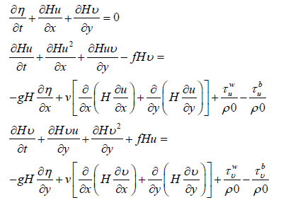
Where
x, y are the horizontal coordinates
t is the time
u=u(x,y,t) is the depth averaged velocity in the x-direction
v=v(x, y,t) is the depth averaged velocity in the y-direction
H=H(x, y,t) is the depth water
ν is the horizontal viscosity
g is the gravity
f =1.01 × 10⁻⁴ rad/s is the Coriolis force.
ρ0=1033 kg/m3 is the density.
η is the water level
is the bottom stress and is the wind stress.
This model is based on the use of explicit center finite difference meth in space and leapfrog scheme with Asselin-Roberts filter in time using open boundary condition, bilinear interpolated and updating by averaging method.
Algorithm of two-way nesting when the space refinement factor is 1:5 and temporal factor is 1:2
Suppose all values in the fine and the coarse meshes are known at time level t=n∆t and we need to find the values of the fine and the coarse meshes in the next time step t=(n+1) ∆t.
(a) In the coarse domain:
1. Get  by solving continuity equation using
  and
and  at time level n.
2. Get and  using and and
  by solving the momentum equations
3. Get  and
and  using
using  by solving momentum equations
(b) In the fine domain:
1. Get  using,
  by solving continuity equation.
2. Solve momentum equations for  and
and  using
using  .
.
3. Get  using
using  by solving continuity equation.
4. Solve momentum equations for  and using .
5. Transferee the results for  and
and  from fine to coarse meshes.
Model Results
Here, we apply a multiple-nested for 2D shallow water equations in case structured grids by using explicit difference method and leapfrog with Asselin-Roberts filter schemes with open boundary conditions, linear interpolation and updating by using average scheme, discusses several examples when the space refinement ratio 1:5 and temporal ratio is 1:2. The results show the performance of nesting technique [8-10].
Case 1: The space refinement ratio is 1:5 and the temporal refinement ratio is 1:2
Example 1:
In this example, we use system for the 2D shallow water equations in nonlinear case with non-rotate f=0 and wind stress=0 to find relative error (RE) l2 to η in case a coarse mesh contain four fine meshes in level 2 at difference times t=500,1000,2000,..4000, 5000 sec when the mesh length 10 × 10.
The following figures show RE l2 in two-way nesting between level 1 and level 2 between different meshes (Figures 1-3 and Table 1).

Figure 1: Shows RE l2 between level 1 and level 2 (mesh 21).

Figure 2: Shows RE l2 between level 1 and level 2 (mesh 21 and mesh 24).

Figure 3: Shows RE l2 between level 1 and level 2 (mesh 21 and mesh 23).
| Information | mesh (01) | mesh (21) | mesh(22) | mesh (23) | mesh (24) |
|---|---|---|---|---|---|
| no.of mesh | 100 × 100 | 100 × 100 | 100 × 100 | 100 × 100 | 100 × 100 |
| length mesh size | 10 | 2 | 2 | 2 | 2 |
| coarse mesh | non | mesh 01 | mesh 01 | mesh 01 | mesh 01 |
| ratio mesh size | non | 5 | 5 | 5 | 5 |
| time step | 0.025 | 0.0125 | 0.0125 | 0.0125 | 0.0125 |
| SWEs | non-linear | non-linear | non-linear | non-linear | non-linear |
| Latitude (North-south) | 1-100 | 41-60 | 81-100 | 11-30 | 61-80 |
| longitude (East-west) | 1-100 | 11-30 | 81-100 | 11-30 | 61-80 |
| CFL condition | — | 0.7 | 0.7 | 0.6 | 0.6 |
Table 1: The information on the establishment of the different meshes (01, 21, 22, 23, 24) for the 2D non-linear shallow water equations.
Example 2:
Here, we use system for the nonlinear 2D shallow water equations with f=0 and wind stress=0 to find RE l2 of free surface in case a coarse mesh contain one fine mesh and a fine mesh in level 2 contain again one fine mesh in level 3 also, a fine mesh in level 3 contains again a fine mesh in level 4 at difference times t=500, 1000, 2000,…4000, 5000 s
The following figures show RE l2 for the free surface between (level (1)-level (2) (mesh 21)) and level (2) - level (3) (mesh 32), (level (2)-level (Figures 4 and 5 and Table 2).

Figure 4: Figure represent the RE between level (1), level (2) and level (2), level (3) mesh 32.

Figure 5: Figure represent RE between level 1, level 2, level 2, level 3 mesh 32 and level 3, level 4 mesh 43.
| Information | mesh (01) | mesh (21) | mesh (32) | mesh (43) |
|---|---|---|---|---|
| Number of meshs | 100 × 100 | 100 × 100 | 100 × 100 | 100 × 100 |
| length mesh size | 10 | 2 | .40 | 0.08 |
| coarse mesh | non | mesh 01 | mesh 21 | mesh 32 |
| mesh size ratio | non | 5 | 5 | 5 |
| time step | 0.025 | 0.0125 | 0.00625 | 0.003125 |
| SWEs | non-linear | non-linear | non-linear | non-linear |
| Latitude (North-south) | 1-100 | 41-60 | 11-30 | 41-60 |
| longitude (East-west) | 1-100 | 11-30 | 11-30 | 41-60 |
| CFL condition | — | 0.7 | 0.7 | 0.6 |
Table 2: The information on the establishment of different meshes (01, 21, 32, 43) for the 2D shallow water equations in non-linear case.
Example 3:
We use system for the nonlinear 2D shallow water equations with f=0 and wind stress=0, to find RE l2 of free surface in case a coarse mesh contains a fine mesh (mesh 24) and a fine mesh in level 2 contain again two fine meshes (mesh 31, mesh 33) in level 3 also, the fine mesh in level 3 contain again a fine mesh (mesh 41) in level 4 with difference times t=500, 1000, 2000,...4000, 5000 s.
The following figures show the RE l2 for the free surface between (level 1-level 2 (mesh 24) and level 2-level 3 (mesh 33)), (level 2-level 3 (mesh 33) and level 3-level 4 (mesh 43)) (Figures 6 and 7 and Table 3).

Figure 6: Shows the REl2 for the free surface in level 1, level 2 (mesh 24) and level 2, level 3 (mesh 33).

Figure 7: Shows RE l2 for the free surface in level 1, level 2 (mesh 24), level 2, level 3 (mesh 33 ) and level 3, level 4 mesh 44.
| Information | mesh (01) | mesh (24) | mesh (31) | mesh (33) | mesh (41) |
|---|---|---|---|---|---|
| No of meshes | 100 × 100 | 100 × 100 | 100 × 100 | 100 × 100 | 100 × 100 |
| mesh size | 10 | 2 | 0.40 | 0.40 | 0.08 |
| coarse mesh | non | mesh 01 | mesh 24 | mesh 24 | mesh 33 |
| mesh size ratio | non | 5 | 5 | 5 | 5 |
| time step | 0.025 | 0.0125 | 0.00625 | 0.00625 | 0.003125 |
| SWEs | non-linear | non-linear | non-linear | non-linear | non-linear |
| Latitude | 1-100 | 61-80 | 61-80 | 41-60 | 31-50 |
| longitude | 1-100 | 61-80 | 11-30 | 41-60 | 31-50 |
| CFL | — | 0.7 | 0.7 | 0.6 |
Table 3: The information on the establishment of the various meshes (01, 24, 31, 33, 31) for the non-linear 2D shallow water equations.
Example 4:
In this example, we use system for the non-linear 2D shallow water equations with f=0 and wind stress=0 to find the RE l2 of free surface in case a coarse mesh contains one fine mesh and a fine mesh in level 2 contains again fine mesh in level 3 also, the fine mesh in level 3 contains again a fine mesh in level 4 at difference times t=500, 1000, 2000,…4000, 5000 s when the water depth constant, the space refinement ratio in level (2,3) is 1:5 and the space refinement ratio in level 4 with mesh (42) is 1:3.
The following figures show RE l2 for the free surface between (level 1-level 2 (mesh 23) and level 2-level 3 (mesh 34)), (level 2-level 3(mesh 32) and level 3-level 4 (mesh 41, mesh 42) (Figures 8 and 9 and Table 4).

Figure 8: ShowS RE l2 between level 1, 2 (mesh 23) - level 2, 3 (mesh 34)) and level 3, 4 (mesh 41).

Figure 9: Shows RE l2 between level 1, level 2 (mesh 23) - level 2, level 3 (mesh 34)) and level 3, level 4 (mesh 42).
| Information | mesh 01 | Mesh 23 | Mesh 34 | mesh 41 | mesh 42 |
|---|---|---|---|---|---|
| Number of meshes | 100 × 100 | 100 × 100 | 100 × 100 | 100 × 100 | 100 × 100 |
| length mesh size | 10 | 2 | 0.40 | 0.133 | 0.133 |
| coarse mesh | non | mesh 01 | mesh 23 | mesh 34 | mesh 34 |
| mesh size ratio | non | 5 | 5 | 5 | 5 |
| time step | 0.025 | 0.0125 | 0.00625 | 0.00625 | 0.003125 |
| SWEs | non-linear | non-linear | non-linear | non-linear | non-linear |
| Latitude (North-south) | 1-100 | 11-30 | 41-60 | 31-50 | 61-80 |
| longitude (East-west) | 1-100 | 11-30 | 41-60 | 31-50 | 41-60 |
| CFL condition | — | 0.7 | 0.7 | 0.6 | 0.6 |
Table 4: The information on the establishment of the various meshes (01, 23, 34, 41, 42) for the non-linear 2D shallow water equations.
Case 1: 2D linear shallow water equations
Example 5:
In this example, we use system for the 2D linear shallow water equations with f=0 and wind stress=0 to find RE l2 of free surface in case a coarse mesh contains four fine meshes at difference times t=500, 1000, 2000,...4000, 5000 s.
The following figures show the RE l2 for the free surface between (coarse mesh and mesh 21 in level 2), (coarse mesh and mesh (22) in level 2), (coarse mesh and mesh (23) in level 2) and (coarse mesh) (Figures 10 and 11 and Table 5).

Figure 10: Show the RE l2 between level 1 and two fine meshes (mesh 21 and mesh 22).

Figure 11: Show the RE l2 between level 1 and two fine meshes (mesh 21, mesh 22, mesh 23 and mesh 24).
| mesh 01 | mesh 21 | mesh 22 | mesh 23 | mesh 24 |
|---|---|---|---|---|
| 100 × 100 | 100 × 100 | 100 × 100 | 100 × 100 | 100 × 100 |
| 10 | 2 | 2 | 2 | 2 |
| – | mesh 01 | mesh 01 | mesh 01 | mesh 01 |
| – | 5 | 5 | 5 | 5 |
| 0.025 | 0.0125 | 0.0125 | 0.0125 | 0.0125 |
| linear | linear | linear | linear | linear |
| 1-100 | 41-60 | 61-80 | 11-30 | 61-80 |
| 1-100 | 11-30 | 61-80 | 11-30 | 61-80 |
| – | 0.7 | 0.7 | 0.6 | 0.6 |
Table 5: The information on the establishment of the various meshes (21, 22, 23, 24) for the non-linear 2D shallow water equations.
Example 6:
In this example, we use system for the 2D linear shallow water equations with f=0 and wind stress=0 to find RE l2 of free surface in case a coarse mesh contains one fine grid and a fine grid in level 2 contains again a fine grid in level 3 also, a fine grid in level 3 contains again a fine grid in level 4 at difference times t=500, 1000, 2000,..4000, 5000 s when the grid length 10 × 10 and the time step in a fine grid is one half time in a coarse grid using open boundary conditions, linear interpolation and average updating procedure.
The following figure show RE l2 between level 1, level 2, level 3 and level 4 (Figure 12 and Table 6).

Figure 12: Show RE l2 between level 1, level 2 and level 3.
| mesh 01 | mesh 21 | mesh 32 | mesh 43 T |
|---|---|---|---|
| 100 × 100 | 100 × 100 | 100 × 100 | 100 × 100 1,l |
| 10 | 2 | .40 | 0.08 |
| – | mesh 01 | mesh 21 | mesh 32 |
| – | 5 | 5 | 5 |
| 0.025 | 0.0125 | 0.00625 | 0.003125 |
| non-linear | non-linear | non-linear | non-linear |
| 1-100 | 41-60 | 11-30 | 41-60 |
| 1-100 | 11-30 | 11-30 | 41-60 |
| – | 0.7 | 0.7 | 0.6 |
Table 6: The information on the establishment of the various meshes (01, 21, 32, 43) for the non-linear 2D shallow water equations.
Example 7:
In this example, we use system for the 2D linear shallow water equations with f=0 and wind stress=0 to find RE l2 of free surface in case a coarse mesh contains one fine mesh and a fine mesh in level 2 contains again a fine mesh in level 3 also, a fine mesh in level 3 contains again a fine grid in level 4 at difference times t=500, 1000, 2000,...4000, 5000 s (Figure 13 and Table 7).

Figure 13: show RE l2 between level 1, level 2, level 3 and level 4.
| Information | mesh 01 | mesh 22 | mesh 31 | mesh 33 | mesh 44 |
|---|---|---|---|---|---|
| Number of meshes | 100 × 100 | 100 × 100 | 100 × 100 | 100 × 100 | 100 × 100 |
| length mesh size | 10 | 2 | 0.40 | 0.40 | 0.08 |
| coarse mesh | non | mesh 01 | mesh 22 | mesh 22 | mesh 33 |
| mesh size ratio | non | 5 | 5 | 5 | 5 |
| time step | 0.025 | 0.0125 | 0.00625 | 0.00625 | 0.003125 |
| SWEs | non-linear | non-linear | non-linear | non-linear | non-linear |
| Latitude (North-south) | 1-100 | 61-80 | 61-80 | 41-60 | 41-60 |
| longitude (East-west) | 1-100 | 61-80 | 11-30 | 41-60 | 41-60 |
| CFL condition | — | 0.7 | 0.7 | 0.6 | 0.6 |
Table 7: The information on the establishment of the various meshes (01, 22, 32, 33, 44) for the non-linear 2D shallow water equations.
Example 8:
We use system for the nonlinear 2D shallow water equations with f=0 and wind stress=0 to find RE l2 of free surface in case a coarse mesh contains one fine mesh and a fine mesh in level 2 contains again a fine mesh in level 3 also, a fine grid in level 3 contains again a fine meshes in level 4 at difference times t =500, 1000, 2000,…4000, 5000 s (Figures 14 and 15 and Table 8).

Figure 14: Shows RE l2 in level 1, level 2 and level 3.

Figure 15: Shows RE l2 in level 1, level 2, level 3 and level 4.
| Information | mesh 01 | mesh 23 | mesh 34 | mesh 41 | mesh 42 |
|---|---|---|---|---|---|
| Number of meshes | 100 × 100 | 100 × 100 | 100 × 100 | 100 × 100 | 100 × 100 |
| length mesh size | 10 | 2 | 0.40 | 0.133 | 0.133 |
| coarse mesh | non | mesh 01 | mesh 23 | mesh 34 | mesh 34 |
| mesh size ratio | non | 5 | 5 | 5 | 5 |
| time step in sec | 0.025 | 0.0125 | 0.00625 | 0.00625 | 0.003125 |
| SWEs | non-linear | non-linear | non-linear | non-linear | non-linear |
| Latitude (North-south) | 1-100 | 11-30 | 41-60 | 31-50 | 61-80 |
| longitude (East-west) | 1-100 | 11-30 | 41-60 | 31-50 | 41-60 |
| CFL condition | — | 0.7 | 0.7 | 0.6 | 0.6 |
Table 8: The information of the establishment of various meshes (01, 23, 34, 41, 42) for the non-linear 2D shallow water.
Example 9: (Case 1: Coupling (embedding) systems for 2D nonlinear shallow water equations)
In this example, we find RE for 2D nonlinear shallow water equations when (υ, windstress and f=0), when coarse mesh contain only one fine mesh at difference times t = 500, 1000,... 4000 s when nx=ny=120, dx=dy=9, time step=0.020 s in a coarse mesh (the information about the coarse and fine meshes are given in table below :) In this case, a coarse mesh in first-level which contains a state of 2D nonlinear shallow water equations and coupling with the fine mesh in second-level mesh which contains a state of 2D nonlinear shallow water equations, the fine mesh in the third-level which contains a state of 2D (Figure 16 and Table 9).
| mesh 01 | mesh 24 | mesh 33 | mesh 41 |
|---|---|---|---|
| 100 × 100 | 100 × 100 | 100 × 100 | 100 × 100 |
| 10 | 2 | 0.40 | 0.08 |
| non | mesh 01 | mesh 24 | mesh 33 |
| non | 5 | 3 | 3 |
| 0.020 | 0.01 | 0.005 | 0.0025 |
| non-linear | non-linear | non-linear | non-linear |
| 1-100 | 61-80 | 61-80 | 41-60 |
| 1-100 | 61-80 | 11-30 | 41-60 |
| 0.7 | 0.7 | 0.6 | 0.6 I |
Table 9: The information on the establishment of the various meshes (01, 24, 33, 41) for the non-linear 2D shallow water.

Figure 16: Compare of REl2 between level 1, level 2- level 2, level, 3 and level 3, level 4.
Example 10: Case 2 Coupling systems for 2D linear/nonlinear shallow water equations
In this example, we find RE l2 for 2D nonlinear shallow water equation such that ν=0, windstress=0 and f=0, when coarse mesh contain more than one level at difference times t = 500, 1000,...4000 s, when nx=ny=120, dx=dy=9, time step=0.020 s in coarse mesh (the information about the coarse and fine meshes are the same previous example).
In this case, when coarse mesh in first-level which contains a state of 2d nonlinear shallow water equations and coupling with the fine mesh in second-level grid which contains a state of 2D linear shallow water equations and the fine mesh in the third-level which contains a state of 2D nonlinear shallow water equations, the fine mesh in the fourth-level which contains a state of 2D nonlinear shallow water equations (Figure 17).

Figure 17: Compare of RE l2 between level 1, level 2 and level 2, level 3 and level 3, level 4.
Example 11: Case 2 - coupling systems for 2D nonlinear/linear shallow water equations
In this example, we find RE l2 for 2D nonlinear shallow water equations such that υ=0, the wind stress=0, f=0 when coarse mesh contain more than one level at difference times t=500, 1000,...4000 s when nx=ny=120, dx=dy=9, time step=0.020 s in coarse mesh (the information about the coarse and fine meshes are the same example 9).
In this case, when coarse mesh in first-level which contains a state of 2d nonlinear shallow water equations and coupling with the fine mesh in second-level mesh which contains a state of 2D linear shallow water equations and the fine mesh in the third-level which contains a state of 2D linear shallow water equations, the fine mesh in the fourth-level which contains a state of 2D nonlinear shallow water equations (Figure 18).

Figure 18: Compare RE between level 1, 2 – level 2,3 and level 3,4.
Conclusion
This paper dealt with two-way interaction technique between coarse and fine grids for the 2D shallow water equations and a new approach is presented to treat this problem. Also, proposed a new two-way interactive algorithm. To verify the efficiency of the nested grid model, some numerical examples are introduced. The accuracy of the nested grid depends on the location of the open boundaries of the nested domains. Boundaries should be located in areas of the coarse grid domain where high accuracy to minimize the error being passed from coarse to fine grids. It was showed the performance techniques using two-way nesting. Two-way nesting ensures dynamical consistency between a coarse mesh and fine mesh happens often. Good results are observed mostly.
References
- Shuto N, Imamura F, Goto C (1988) Numerical simulation of the transoceanic propagation of tsunamis. The Sixth Congress of the Asian and Pacific Regional Division, Int Assoc Hydraul Res, Kyoto, Japan.
- Wang X, Liu PLF (2007) Numerical simulations of the 2004 Indian Ocean tsunamis - coastal effects. J Earthq Tsunami 1: 273297.
- Wang X, Liu PLF (2006) An analysis of 2004 Sumatra earthquake fault plane mechanisms and Indian Ocean tsunami. J Hydraulic Res 44: 147154.
- Wang X (2007) User manual of COMCOT. Cornell University, New York, USA.
- Woo SB, Liu PLF, Cho YS (1998) Computer programs for tsunami propagation and inundation. Technical report, Cornell University, New York, USA.
- Kantha LH, Clayson CA (2000) Numerical Models of Oceans and Oceanic Processes. Elsevier, UK.
- Garcia-Navarro P, Burguete J, Brufau P, Murillo J (2008) The shallow water equations: An example of hyperbolic system. Real Academia de Ciencias de Zaragoza 31: 81-119.
- Rothstein LM, Ginis I, Richardson RM (1997) Design of a multiply nested primitive equation ocean model. Mon Weather Rev 126: 1054-1079.
- Allen JS, Pullen J (2001) Modelling studies of the coastal circulation of the northern coast of California: statistics and patterns of wintertime flow. J Geophys Res 26: 959-926
- Spall MA, Robinson AR (1989) A hybrid coordinate open ocean primitive equation model. Math Comput Simul 31: 241-269.