Spanish
  Chinese
  Russian
  German
  French
  Japanese
  Portuguese
  Hindi
Hindi Research Article, Res Rep Math Vol: 2 Issue: 1
Enlarging the Radius of Convergence for the Halley Method to Solve Equations with Solutions of Multiplicity under Weak Conditions
Ioannis K Argyros1* and Santhosh George2
1Department of Mathematical Sciences, Cameron University, Lawton, OK 73505, USA
2Department of Mathematical and Computational Sciences, NIT Karnataka, India
*Corresponding Author : Ioannis K Argyros
Department of Mathematical Sciences, Cameron University, Lawton, OK 73505, USA
Tel: (580) 581-2200
E-mail: iargyros@cameron.edu
Received: August 18, 2017 Accepted: January 15, 2018 Published: February 10, 2018
Citation: Argyros IK, George S (2018) Enlarging the Radius of Convergence for the Halley Method to Solve Equations with Solutions of Multiplicity under Weak Conditions. Res Rep Math 2:1
Abstract
The objective of this paper is to enlarge the ball of convergence and improve the error bounds of the Halley method for solving equations with solutions of multiplicity under weak conditions.
Keywords: Halley’s method; Solutions of multiplicity; Ball convergence; Derivative; Divided difference
Introduction
Many problems in applied sciences and also in engineering can be written in the form like
f (x) = 0, (1.1)
Using mathematical modeling, where  is sufficiently many times differentiable and D is a convex subset in
  . In the present study, we pay attention to the case of a solution p of multiplicity m>1; namely
  and
and 
The determination of solutions of multiplicity m is of great interest. In the study of electron trajectories, when the electron reaches a plate of zero speed, the function distance from the electron to the plate has a solution of multiplicity two. Multiplicity of solution appears in connection to Van Der Waals equation of state and other phenomena. The convergence order of iterative methods decreases if the equation has solutions of multiplicity m. Modifications in the iterative function are made to improve the order of convergence. The modified Newton’s method (MN) defined for each n=0,1,2,..
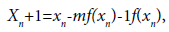 (1.2)
(1.2)
Where x0∈D is an initial point is an alternative to Newton’s method in the case of solutions with multiplicity m that converges with second order of convergence.
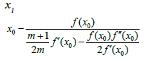
A method with third order of convergence is defined by modified Halley method (MH) [4]
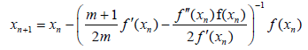 (1.3)
(1.3)
Method (1.3) is an extension of the classical Halley’s method of the third order. Other iterative methods of high convergence order can be found in [1-15] and the references therein.
Let 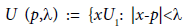 denote an open ball and
  denote its closure. It is said that
 is a convergence ball for an iterative method, if the sequence generated by this iterative method converges to p; provided that the initial point
  But how close x0 should be to x* so that convergence can take place. Extending the ball of convergence is very important, since it shows the difficulty; we confront to pick initial points. It is desirable to be able to compute the largest convergence ball. This is usually depending on the iterative method and the conditions imposed on the function f and its derivatives. We can unify these conditions by expressing them as:
 (1.4)
(1.4)
 (1.5)
(1.5)
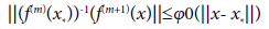
for all x, y ∈ D; where 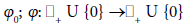 are continuous and nondecreasing functions satisfying
 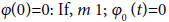 and
and
Then, we obtain the conditions under which the preceding methods were studied [1-17]. However, there are ceases where even (1.6) does not hold (see Example 4.1). Moreover, the smaller functions Õ0, Õ are chosen, the larger the radius of convergence becomes. The technique, we present next can be used for all preceding methods as well as in methods where m=1: However, in the present study, we only use it for MH. This way, in particular, we extend the results in [4,5,12,13,16,17].
The rest of the paper is structured as follows. Section 2 contains some auxiliary results on divided differences and derivatives. The ball convergence of MH is given in Section 3. The numerical examples in the concluding Section 4.
Auxiliary Results
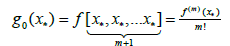
In order to make the paper as self-contained as possible, we restate some standard definitions and properties for divided differences [4,13,16,17].
Definition: The divided differences 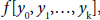 on k+1 distinct points y0, y1,…,yk of a function f(x) are defined by

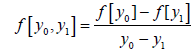
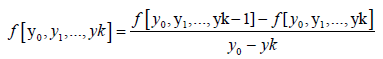 (2.1)
(2.1)
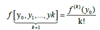
If the function f is sufficiently differentiable, then its divided differences 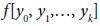 can be defined if some of the arguments yi coincide. for instance, if f(x) has k-th derivative at y0; then it makes sense to define
Lemma: The divided differences f[y0, y1,…, yk] are symmetric functions of their arguments,i.e., they are invariant to permutations of the y0, y1,…, yk.
Lemma: If the function f has k-th derivative, and f (k)(x) is continuous on the interval  then
then
 (2.3)
(2.3)
Where 
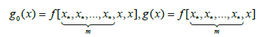
Lemma: If the function f has (k +1)-th derivative, then for every argument x; the following formulae holds
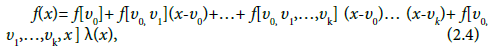
Where
 (2.5)
(2.5)
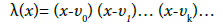
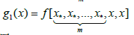
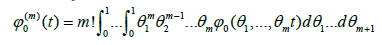
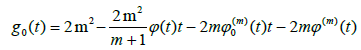
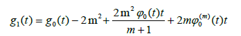
Lemma: Assume the function f has continuous (m + 1)-th derivative, and x* is a zero of multiplicity m; we define functions g0, g and g1 as
 (2.6)
(2.6)
Then,
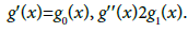 (2.7)
(2.7)
Lemma: If the function f has an (m+1)-th derivative, and x* is a zero of multiplicity m, then for every argument x, the following formulae hold
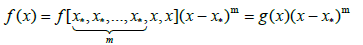 (2.8)
(2.8)
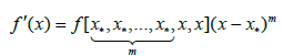
 (2.9)
(2.9)
And

where g0(x); g(x) and g1(x) are defined previously.
Local Convergence
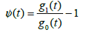
It is convenient for the local convergence analysis that follows to define some real functions and parameters. Define the function ðÂœ“0 on + U{0} by
We have  and
and  Suppose
 positive number of + ∞
for sufficiently large t. It then follows from the intermediate value theorem that function ψ0 has zeros in the interval (0, + ∞): Denote by ρ0 the smallest such zero. Define functions  on the interval
  by
by

And
we get that 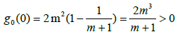 and
and  as
as
Denote by r0 the smallest zero of function g0 in the interval (0, ρ0): Moreover, we get that and
and 
Denote by r the smallest zero of function ðÂœ“ on the interval (0,r0 ): Then, we have that for each t ∈ [0, r)

The local convergence analysis is based on conditions (A):
(A1) Function  times differentiable and x* is a zero of multiplicity m.
(A2) Conditions (1.4) and (1.5) hold
 where the radius of convergence r is defined previously.
(A4) Condition (3.1) holds
Theorem Suppose that the (A) conditions hold. Then, sequence  generated for
  by MH is well defined in U(x*,r), remains in U(x*,r) for each n = 0, 1, 2…and converges to x*
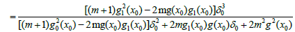
Proof. We base the proof on mathematical induction. Set δn=xn- x* and choose initial point x0∈U(x*,r)- {x*}. Using (1.2), (2.8), (2.9) and (2.10), we have in turn that
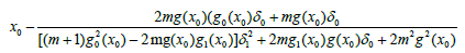 (3.3)
(3.3)
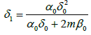
so
 (3.4)
(3.4)
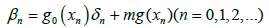
or
 (3.5)
(3.5)
Where

 (3.6)
(3.6)
By (2.2) and (2.6), we can get
 (3.7)
(3.7)
and by the condition (1.4) and
 we obtain,

 (3.8)
(3.8)
where y0 is a point between x0 and x*, so g(x0)≠0
 (3.9)
(3.9)
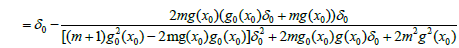
Hence, we get
 (3.10)
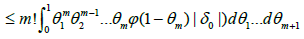
Using (2.2), (2.6), conditions (1.4), (1.5) and Lemma 2.3, we have

 (3.11)
And

 (3.12)
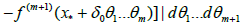

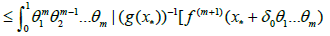
In view of (3.10), (3.11) and (3.12), we obtain
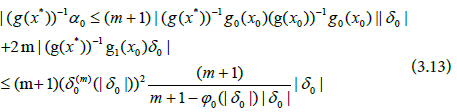
 we get


 (3.14)

We get by (3.8), (3.13) and (3.14)
 (3.15)

Where
 (3.16)
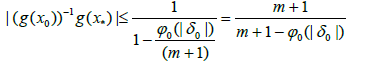
By simply replacing x0, x1 by xk, xk+1 in the preceding estimates, we get
 (3.17)
so 
Next, we present a uniqueness result for the solution x*
Proposition Suppose that the conditions (A) hold. Then, the limit point x* is the only solution of equation 
Proof Let x** be a solution of equation f(x)=0 in D1: We can write by (2.8) that
 (3.18)
Using (1.4) and the properties of divided differences, we get in turn that

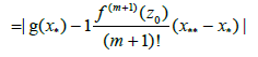 (3.19)
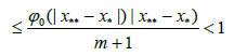
for some point between x** and x* It follows from (3.18) and (3.19) x**= x
Numerical Examples
We present a numerical example in this section.
Example Let D=[0; 1]; m=2; p=0 and define function f on D by
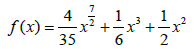
we have 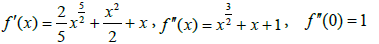
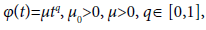
function f ′′ cannot satisfy (1.5) with ðÂœ“ given by (1.6). Hence, the results in [4,5,12,13,16,17] cannot apply. However, the new results apply for  and
and  Moreover, the convergence radius is r=0.8.
Example Let D=[-1, 1], m=2; p=0 and define function f on D by

We get  The convergence radius is r=1:4142; so choose r=1.
References
- Amat S, Hernández MA, Romero N (2012) Semi-local convergence of a sixth order iterative method for quadratic equations. Appl Numer Math 62: 833-841.
- Argyros IK (2007) Computational theory of iterative methods, Elsevier Publ Co, New York, USA.
- Argyros I (2003) On the convergence and application of Newtons method under Holder continuity assumptions. Int J Comput Math 80: 767-780.
- Bi W, Ren H, Wu Q (2011) Convergence of the modified Halley's method for multiple zeros under Holder continous derivatives. Numer Algor 58: 497-512.
- Chun C, Neta B (2009) A third order modification of Newton's method for multiple roots. Appl Math Comput 211: 474-479.
- Hansen E, Patrick M (1977) A family of root finding methods. Numer Math 27: 257-269.
- Magrenan AA (2014) Different anomalies in a Jarratt family of iterative root finding methods. Appl Math Comput 233: 29-38.
- Magrenan AA (2014) A new tool to study real dynamics: The convergence plane. Appl Math Comput 248: 29-38.
- Neta B (2008) New third order nonlinear solvers for multiple roots. Appl Math Comput 202: 162-170.
- Obreshkov N (1963) On the numerical solution of equations (Uulgarian). Annuaire Univ Sofa fac Sci Phy Math 56: 73-83.
- Osada N (1994) An optimal mutiple root finding method of order three. J Comput Appl Math 52: 131-133.
- Petkovic M, Neta B, Petkovic L, Dzunic J (2012) Multipoint methods for solving nonlinear equations, Elsevier, Netherlands.
- Ren H, Argyros IK (2010) Convergence radius of the modified Newton method for multiple zeros under Holder continuity derivative. Appl MathComput 217: 612-621.
- Schroder E (1870) Uber unendlich viele Algorithmen zur Auosung der Gieichunger. Math Ann 2: 317-365.
- Traub JF (1982) Iterative methods for the solution of equations. AMS Chelsea Publishing, USA.
- Zhou X, Song Y (2011) Convergence radius of Osada's method for multiple roots under Holder and Center-Holder continous conditions. AIP Conf Proc 1389: 1836-1839.
- Zhou X, Chen X, Song Y (2014) On the convergence radius of the modified Newton method for multiple roots under the center- Holder condition. Numer Algor 65: 221-232.