Research Article, Res Rep Math Vol: 1 Issue: 1

From Configurations to Branched Configurations and Beyond

Jean-Pierre Magnot^*

Department of Forestry and Biodiversity, Tripura University, Suryamaninagar, Agartala, India

*Corresponding Author : Jean-Pierre Magnot
Department of Mathematics, University of Angers, Lycee Jeanne dArc, 30 avenue de Grande Bretagne, F-63000, Clermont-Ferrand, France
Tel: +33 2 41 96 23 23
E-mail: jean-pierr.magnot@ac-clermont.fr

Received: July 19, 2017 Accepted: October 18, 2017 Published: November 02, 2017

Citation: Magnot JP (2017) From Configurations to Branched Configurations and Beyond. Res Rep Math 1:1

Abstract

Keywords: Finite and infinite configuration spaces; Branched dynamics

Introduction

Finite and infinite configuration spaces are rather old topics, see e.g. [1,2] and the references cited therein, that had many applications in various settings in mathematical physics and representation theory. More recently, several papers, including [3-6] showed how these topics could be applied in various disciplines: ecology, financial markets, and so on. This large spectrum of applications principally comes from the simplicity of the model: considering a state space N, finite or infinite configurations are finite or countable sets of values in N: This is why we begin with giving a short description of this setting, and describe a differentiable structure that can fit with easy problems of dynamics. This structure, which can be seen either as a Frölicher structure or as a diffeological one, is carefully described and the links between these two frameworks are summarized in the appendix. We also give a result that seems forgotten in the past literature: the infinite configuration space used in e.g. [7] is an infinite dimensional manifold.

But the main goal of this paper is to include one dimensional turbulence effects (in particular period doubling, see e.g. [8]) in the dynamics described by finite or infinite configuration spaces. For this, we change the metric into the Hausdorff metric. This enables to “glue together” two configurations into another one and to describe shocks. Therefore, the dynamics on this modified configuration space are described by multivalued paths that are particular cases of graphs on N; which explains the terminology: “branched configuration”.

We finish with the description of the configurations used e.g. in optimal transport, the space of probability measures, and shows how they can also furnish configurations for uncompressible fluids. In these settings, branching effects are well-known and sometimes obvious, and we do not need any adaptation of the framework to obtain a full description of them. Therefore, what we call branched configurations appears as an intermediate (an we hope useful) step between dynamics of e.g. a N-body problem and e.g. wave dynamics.

Dirac configuration spaces on a locally compact manifold

Let us describe step by step a way to build infinite configurations, as they are built in the mathematical literature. We explain each step with the configurations already defined in e.g. Albeverio et al. [7] and Fadell et al. [1], the generalization will be discussed later in this paper.

A set of I -configurations is a set of objects that are modelizations of physical quantities. For example, in the settings [1-6], the physical quantity modeled is the position of one particle. The whole world is modeled as a locally compact manifold N, and the set of 1-configurations is itself N, or equivalently the set of all Dirac measures on N.

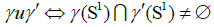
Let I be a set of indexes. I can be countable or uncountable. We define the indexed (or the ordered if I isequipped with its total order) configuration spaces. For this, we need to define a symmetric binary relation relation u on Γ¹, that expresses the compatibility of two physical quantities. We assume also that u has the following property:

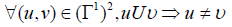
In the settings Albeverio et al. [7] and Finkelshtein et al. [1], two particles cannot have the same position. Then, for x, y ∈ N [2],

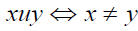
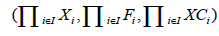
With these restrictions, we can define the indexed or ordered configuration spaces:

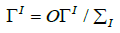
The general configuration spaces are not ordered. Let Σ_n be the group of bijections on , and Σ_I be the set of bijections on I. We can define two actions:

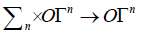
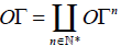
and its infinite analog:

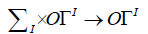
where Σ_I is a subgroup of the group of bijections of I: In the sequel, I is countable with discrete topology, which avoids topological problems on Σ_I as in more complex examples. Then, we define general configuration spaces:

Configuration spaces on more general settings

In the machinery of the last section, the properties of the base manifold N are not used in the definition of the space Γ¹. This is why the starting point can be Γ¹ instead of N, and we can give it the most general differentiable structure. Let us first consider the most general case [9]:

Proposition 1.1: If Γ¹ is a diffeological space, then Γⁿ, Γ and Γ^I are diffeological spaces

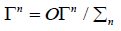
Proof: (Γ¹)ⁿ (resp. (Γ¹)^N) is a diffeological space according to Proposition 4.8 (resp. Proposition 4.10), so that, OΓⁿ (resp. OΓ^I) is a diffeological space as a subset of (Γ¹)ⁿ (resp. (Γ¹)^N). Thus, Γⁿ = Oⁿ/ Σ_n (resp. Γ¹ = O_n/Σ) has the quotient diffeology by Proposition 4.12, which ends the proof.

Let us now turn to the cases where Γ^I has a stronger structure. We already know that Γn is a manifold if Γ¹ is a manifold.

Proposition 1.2: If Γ¹ is a Frölicher space, then Γⁿ (and hence Γ) is a Frölicher space.

Proof: Adapting the last proof, using Proposition 4.9 instead of Proposition 4.8, we get that OΓⁿ is a Frolicher space if Γ¹ is a Frolicher space. Let us now build a generating set of functions for the Frolicher structure on OΓⁿ. Let f: be a smooth map. We define the symmetrization of f:

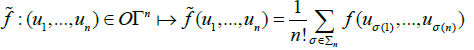
The set of functions generate the contours on OΓⁿ, and then, passing to the quotient, generate the contours on Γⁿ

Setting a Frölicher structure on indexed configurations is only a straightforward consequence of Proposition 4.10:

Proposition 1.3: If Γ¹ is a Frölicher space, then OΓ^I is a Frölicher space.

But the problem of a Frölicher structure on Γ^I a little bit more complicated; let us explain why and give step by step the construction of the Frölicher structure. We first notice that the contours of the Frölicher push forward naturally by the quotient map ut, if one wants to describe a generating set of functions, by Proposition 4.9, one has to consider all combinations of a finite number of smooth functions This generating set does not contain any Σ_I -invariant function, except constant functions. This is why the approach used in the proof of the Proposition 1.2 cannot be applied here. For this, one has to consider the set

of equivariant functions on OΓ^I: This discusssion can become very quickly naïve and we prefer to leave this question to more applied works in order to fit with known examples instead of dealing with too abstract considerations.

Topological Configuration Spaces

In this section, we present examples of 1-configurations and their associated configuration spaces. Manifolds will replace the Dirac measures used in Albeverio et al. [7]. In the sequel, N is a Riemannian smooth locally compact manifold. The 1-configurations considered keep their topological properties, as in the model of elastodymanics (see e.g. Hughes et al. [10]) or in various quantum field theories. Notice also that we do not give compatibility conditions between two 1-configurations: we would like to give the more appropriate conditions in order to fit with the applied models, this is why we leave this point to more specialized works.

Topological 1-configurations

We follow here, for example, Hughes T et al. [10].

Definition 2.1: Let M be a smooth compact manifold and N an arbitrary manifold. We set

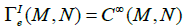
One can also only consider embeddings, and set:

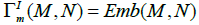
where dimM<dimN, and Emb is the set of embeddings. The things run as in the first case, since 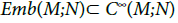is an open subset of

Examples of topological configurations

Links. Let 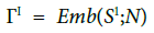Here, we fix the uncompatibility relation as

Then, is the space of n→links of class C^k, which is a Frechet manifold.

Triangulations: Consider the n-simplex

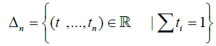
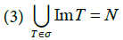
If N is a n-dimensional manifold, a (finite) triangulation σ of N is such that:

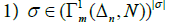
(2) Let such that T≠ T′ then is a simplex or a collection of simplexes of each border Im(∂T) and Im :

We get by condition 2 a compatibility condition u; for which we can build and If N is compact, the set of triagulations of N is a subset of If N is non compact and locally compact, the set of triangulations of N is a subset of

More generally, for p≤n; one can build and This example will be discussed in the section 3.

Strings and membranes: A string is a smooth surface Σ possibly with boundary, embedded in A membrane is a manifold M of higher dimension embedded in some We recover here some spaces of the type which will be also discussed in section 3.

Branched Configuration Spaces

Dirac branched configurations

As we can see in section 1.1, finite configurations Γare made of a countable disjoint union. We now fix a metric d on N: The idea of branched configurations is to glue together the components Γⁿ on the generalized diagonal, namely, we define the following distance on Γ:

Definition 3.1: Let

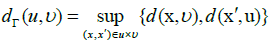
Proposition 3.2: d_Γ is a metric on Γ:

Proof: We remark that d_Γ is the Hausdorff distance restricted to Γ:

The following proposition traduces the change of topology of Γ into BΓ by cutand paste property:

Proposition 3.3: where the identification is made along the trace on Γⁿ⁺¹ of the d_Γ - neighborhoods of in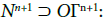

We remark that we can also define a Frolicher structure on BΓ with generating set of functions the set

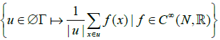
This structure will be recovered later in this paper.

Examples of topological branched configurations

The path space, branched paths and graphs: Let

be the space of smooth paths on N: A γ path has a natural orientation, and has a beginning α(γ) and an end ω(γ): We define a compatibility condition

and we remark that the set of piecewise smooth paths on N is a subset of saying that is a piecewise smooth path if and only if

This relation, stated from the natural definition of the composition * of the groupoid of paths, is not unique and can be generalized.

Definition 3.4: Let and let We define the equivalence relation ∼ by

The maps and extends to \set theorical” maps and The following is now natural:

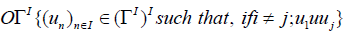
Definition 3.5: A branched path is an element γ of such that, if

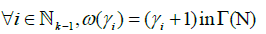
Example: Let us consider the following paths :

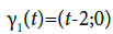
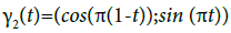
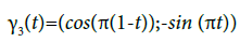
Then,

And

This shows that

is a branched path of

Alternate approach to branched paths: branched sections of a fiber bundle.

Let be a fiber bundle of typical fiber F₀:

Here, Let be a fiber bundle over M with typical fiber F₀: Let

This is trivially a fiber bundle of basis M with typical fiber

Definition 3.6: A non-section of F is a section of which cannot be decomposed into n sections of F.

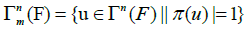
We define also 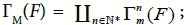and also the non sections based of Γ^I(F₀): We can define the same way BΓ_M(F) using the branxhed configuration space instead of the configuration space, since the definitions from the set-theoric viewpoint are the same.

(Toy) Example: Let us consider the following example: {up; down}, and {{up; {down}; {up; down}}; that models the position of an electron in the 3-dimensional space , associated to its spin. When the electron spin cannot be determined (i.e. out of the action of adequate electromagnetic fields), the picture proposed by Schrodinger is to consider that its spin is both up and down (this picture is also called the \Schrodinger cat” when we replace \up” and \down” by \dead” and \alive”).

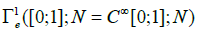
Let us now consider the Frolicher structure described on section 3.1. It is based on the natural diffeology carried by each and by the set of paths ' P₁ that are paths 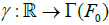such that

is a smooth path on

is a smooth path on

Let Then for any smooth map

where c are the trajectories going to l in 0- equals to the sum of the infinite jet of

where c+ are the trajectories coming from l in 0⁺:

Remark that the last condition comes from the smoothness required for each map with This fits with the (fiberwise) frolicher structure of BΓ(F₀): Then, a finitely branched section of F is a smooth section of The first examples that come to our mind are the well-known branched processes, and we can wonder some deterministic analogues replacing stochastic processes by dynamical systems. Let us here sketch a toy example extracted from the theory of turbulence:

Example: equilibum of mayies population Assuming that Mayies live and die in the same portion of river, the population p_n+1 at the year (n+1) is obtained from the population p_n at the year n (after normalization procedure) by the formula

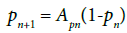
where A ∈ [0; 4] is a constant coming from the environmental data. For A small enough, the fixed point of the so-called “logistic map” is stable, hence the population p_n tends to stabilize around this value. But when A is increasing, the fixed point becomes unstable and p_n tends to stabilize around 2^k multiple values which are the stable fixed points of the map obtained by composition rule.

Now, assume that we consider a river (or a lake), modelized by an interval (or an open subset of that we denote by U, where the parameter A is a smooth map U → [0; 4]: The parameter A is a smooth map U → [0; 4] and the cardinality of configuration of equilibrum depends on the value of A:

Non sections in higher dimensions: The example of a lake where mayflies live and die gives us a nice example of branched surface viewed as an element of The same procedure can be implemented in gluing simplexes, or strings or membranes along their borders to get branched objects, but we prefer to postpone this problem to a work in progress where links with stochastic objects should be performed.

Measure-Like Configurations: An Example at the Borderline of Branched Configurations and Dynamics on Probability Spaces

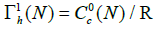
Dynamics on probability space is a fast-growing subject and is shown to give rise to branched geodesics [11]. Following the same procedure as for branched topological configurations, we show her how a restricted space fits with particular goals. The goals described he1re are linked with image recognition for the configuration space above, and to uncompressible fluid dynamics when we equip with the diffeology P₀ of constant volume above. Let C⁰_c be the set of compactly supported valued smooth maps on N. We define the relation of equivalence R by:

Let us first give the definition of the set of 1-configurations:

Definition 4.1: We set

Such a space is not a manifold, but we show that it carries a natural diffeology. is a topological vector space, and hence carries a natural diffeology P₀. We define the following:

Definition 4.2: Let be the set of P₀-plots such that, for any open subset A with compact closure A of N, for any open subset O′ of O such that if

the map

is constant on O′, where Vol is the Riemannian volume.

This technical condition ensures that the volume of any connected component of the support of p(x) is constant. P₁ is obviously a diffeology on , and we can state

Proposition 4.3: Let 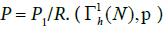is a diffeological space.

The proof is a straightforward application of Definition 4.12. It seems difficult to give this space a structure of Frölicher space, or even a natural topology except the topology of vague convergence of measures, which is not the topology induced by the diffeology we have defined. As a consequence, we can only state that the welldefined configuration spaces Γ and Γ^I are diffeological spaces. The technical conditions of Definition 4.2 ensures that volume preserving is a consequence of smoothness with respect to P1; and hence is particularily designed for (viscous) uncompressible fluid dynamics. A 1-confiuguration can have many connected components, and therefore branching effects are included in the definition of 1-configurations. One could understand n-configurations as the presence of n (non mixing) fluids.

Appendix: Preliminaries on Differentiable Structures

The objects of the category of -finite or infinite- dimensional smooth manifolds is made of topological spaces M equipped with a collection of charts called maximal atlas that enables one to make differentiable calculus. But there are some examples where a differential calculus is needed whereas no atlas can be defined. To circumvent this problem, several authors have independently developped some ways to define differentiation without defining charts. We use here three of them. The first one is due to Souriau [12], the second one is due to Sikorski, and the third one is a setting closer to the setting of differentiable manifolds is due to Frölicher (see e.g. Cherenack P et al. [13] for an introduction on these two last notions). In this section, we review some basics on these three notions.

Souriau’s Diffeological Spaces, Sikorski’s Differentiable Spaces, Frolicher Spaces

Definition 4.4: Let X be a set.

A plot of dimension p (or p-plot) on X is a map from an open subset to X.

A diffeology on X is a set P of plots on X such that, for all pN, - any constant map is in P;

Let I be an arbitrary set; let 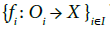be a family of maps that extend to a map 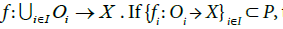then (chain rule) Let f∈P, defined on . Let an open subset of Rq and g a smooth map (in the usual sense) from O′ to O. Then,

If P is a diffeology X, (X;P) is called diffeological space. Let (X;P) et (X′;P′) be two diffeological spaces, a map f : X → X′ is differentiable (=smooth) if and only if f(P) ⊂ P’.

Remark: Notice that any diffeological space (X,P) can be endowed with the weaker topology such that all the maps that are in P are continuous. But we prefer to mention this only for memory as well as other questions that are not closely related to our construction, and stay closer to the goals of this paper. Let us now define the Sikorski’s differential spaces. Let X be a Haussdorf topological space.

Definition 4.5: A (Sikorski’s) differential space is a pair (X;F) where F is a family of functions such that

the topology of X is the initial topology with respect to F

- for any n ∈ N, for any smooth function , for any

Let (X;F) et (X′;F′) be two differential spaces, a map f: X→ X′ is differentiable (=smooth) if and only if

We now introduce Frölicher spaces.

Definition 4.6: A Frölicher space is a triple (X;F; C) such that - C is a set of paths

- A function is in F if and only if for any

- A path is in C (i.e. is a contour) if and only if for any .

Let (X;F;C) et (X′;F′;C′) be two Frölicher spaces, a map f : X → X′ is differentiable (=smooth) if and only if

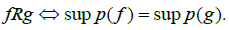
Any family of maps F_g from X to generate a Frolicher structure (X;F; C), setting [14]:

Such that

Such that

One easily see that This notion will be useful in the sequel to describe in a simple way a Frolicher structure.

A Frölicher space, as a differential space, carries a natural topology, which is the pull-back topology of via F. In the case of a finite dimensional differentiable manifold, the underlying topology of the Frölicher structure is the same as the manifold topology. In the infinite dimensional case, these two topologies differ very often.

In the three previous settings, we call X a differentiable space, omitting the structure considered. Notice that, in the three previous settings, the sets of differentiable maps between two differentiable spaces satisfy the chain rule. Let us now compare these three settings: One can see (see e.g. [13]) that we have the following, given at each step by forgetful functors:

smooth manifold ⇒ Frölicher space ⇒ Sikorski differential space

Moreover, one remarks easily from the definitions that, if f is a map from a Frölicher space X to a Frölicher space X′, f is smooth in the sense of Frölicher if and only if it is smooth in the sense of Sikorski.

One can remark, if X is a Frölicher space, we define a natural diffeology on X by Magnot [15]:

p-paramatrization on (in the usual sense) }.

With this construction, we get also a natural diffeology when X is a Frölicher space. In this case, one can easily show the following:

Proposition 4.7: Let (X;F;C) and (X′;F′;C′) be two Frölicher spaces. A map f : X → X′ is smooth in the sense of Frölicher if and only if it is smooth for the underlying diffeologies [15].

Thus, we can also state:

smooth manifold ⇒ Frölicher space ⇒ Diffeological space

Cartesian Products

The category of Sikorski differential spaces is not cartesianly closed, see e.g. [13]. This is why we prefer to avoid the questions related to cartesian products on differential spaces in this text, and focus on Frölicher and diffeological spaces, since the cartesian product is a tool essential for the definition of configuration spaces.

In the case of diffeological spaces, we have the following [12,16-19]:

Proposition 4.8: Let (X;P) and (X′;P′) be two diffeological spaces. We call product diffeology on XxX′ the diffeology P x P′ made of plots g: O → XxX′ that decompose as g = f x f ′, where f : O → X ∈ P and f ′: O → X′ ∈ P′.

Then, in the case of a Frölicher space, we derive very easily, compare with e.g. Kriegl A et al. [14]:

Proposition 4.9: Let (X;F;C) and (X′;F′;C′) be two Frölicher spaces, with natural diffeologies P and P′ . There is a natural structure of Frölicher space on XxX′which contours C x C′ are the 1-plots of P x P′.

We can even state the following results in the case of infinite products.

Proposition 4.10: Let I be an infinite set of indexes, that can be uncoutable.

(adapted from [21] ) Let be a family of diffeological spaces indexed by I. We call product diffeology on the diffeology made of plots that decompose as

where This is the biggest diffeology for which the natural projections are smooth.

Let 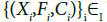be a family of Frolicher spaces indexed by I, with natural diffeologies P_i. There is a natural structure of Frölicher space

which contours are the 1-plots of A generating set of functions for this Frölicher space is the set of maps of the type:

where J is a finite subset of I and φ is a linear map

Proof: By definition, following [12,20], is the biggest diffeology for which natural projections are smooth. Let g: O→ X_i be a plot.

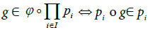
where p_i is the natural projection onto X_i , which gets the result.

With the previous point and Proposition 4.7, we get the family of contours of the product Frölicher space.

Push-Forward, Quotient and Trace

We give here only the results that will be used in the sequel.

Proposition 4.11: Let (X, P) be a diffeological space, and let X′ be a set. Let f : X → X′ be a surjective map. Then, the set [12,21].

f(P) = {u such that u restricts to some maps of the type f o p; p ∈ P} is a diffeology on X′, called the push-forward diffeology on X′ by f .

We have now the tools needed to describe the diffeology on a quotient:

Proposition 4.12: Let (X, P) b a diffeological space and R an equivalence relation on X. Then, there is a natural diffeology on X/R, noted by P/R, defined as the push-forward diffeology on X/R by the quotient projection X → X/R.

Given a subset X₀ ⊂ X, where X is a Frolicher space or a diffeological space, we can define on trace structure on X₀, induced by X.

If X is equipped with a diffeology P, we can define a diffeology P_o on X₀ setting

P₀ = { p ∈ P such that the image of p is a subset of X₀ }.

If (X, F, C) is a Frolicher space, we take as a generating set of maps F_g on X₀ the restrictions of the maps f ∈ F. In that case, the contours (resp. the induced diffeology) on X₀ are the contours (resp. the plots) on X which image is a subset of X₀.

References

1. Fadell ER, Husseini SY (2012) Geometry and topology of configuration spaces. Springer Science & Business Media, USA.
2. Ismagilov RS (1996) Representations of infinite-dimensional groups. American Mathematical Soc.
3. Finkelshtein D, Kondratiev Y, Kutoviy O (2010) Vlasov scaling for stochastic dynamics of continuous systems. J Stat Phys 141: 158-78.
4. Finkelshtein D, Kondratiev Y, Kutoviy O (2012) Semigroup approach to birth-and-death stochastic dynamics in continuum. J Funct Anal 262: 1274-1308.
5. Finkelshtein D, Kondratiev Y, Kozitsky Y, Kutoviy O (2011) Markov evolution of continuum particle systems with dispersion and competition.
6. Finkelshtein D, Kondratiev Y, Kutoviy O (2013) Establishment and fecundity in spatial ecological models: statistical approach and kinetic equations. Infinite Dimensional Analysis, Quantum Probability and Related Topics 16: 1350014.
7. Albeverio S, Daletskii A, Lytvynov E (2001) De Rham cohomology of configuration spaces with Poisson measure. J Funct Anal 185: 240-273.
8. Hilborn R (2012) Chaos an non linear dynamics, Oxford university Press UK.
9. Hagedorn D, Kondratiev Y, Pasurek T, Röckner M (2013) Gibbs states over the cone of discrete measures. J Funct Anal 264: 2550-2583.
10. Hughes T, Marsden JE (1983) Mathematical foundations of elasticity Prentice-Hall Civil Engineering and Engineering Mechanics Series. Englewood Clis, New Jersey, Prentice-Hall, USA.
11. Ohta SI (2014) Examples of spaces with branching geodesics satisfying the curvatureâ�?dimension condition. Bull Lond Math Soc 46: 19-25.
12. Souriau JM (1986) Un algorithme générateur de structures quantiques.
13. Cherenack P, Ntumba P (2001) Spaces with differential structure and an application to cosmology. Demonstr Math 34: 161-180.
14. Kriegl A, Michor PW (1997) The convenient setting of global analysis. American Mathematical Soc, USA.
15. Magnot JP (2008) Difféologie du fibré d’Holonomie en dimension infinite. Math Rep Can Roy Math Soc 28: 121-128.
16. Donato P (1984) Revetements de groupes differentiels These de doctorat detat. Universite de Provence, Marseille, UK.
17. Frölicher A, Kriegl A (1988) Linear spaces and differentiation theory, John Wiley & Sons Inc, USA.
18. Iglesias P (1987) Connexions et diffeologie Aspects dynamiques et topologiques des groupes infinis de transformation de la mecanique Travaux en cours 25: 61-78.
19. Leslie J (2003) On a diffeological group realization of certain generalized symmetrizable Kac-Moody Lie algebras. J Lie Theor 13: 427-442.
20. Lesne A (1996) Méthodes de renormalisation. Phénomènes critiques, chaos, structures fractales, Eyrolles, Paris, UK.
21. Magnot JP (2013) Ambrose–Singer Theorem on Diffeological Bundles and Complete Integrability of the Kp Equation. Int J Geom Methods Mod Phys 10: 1350043.