Spanish
  Chinese
  Russian
  German
  French
  Japanese
  Portuguese
  Hindi
Hindi Research Article, J Hydrogeol Hydrol Eng Vol: 6 Issue: 2
Hydrological Modeling of Musi River Basin, India and Sensitive Parameterization of Streamflow Using SWAT CUP
Srinivas G* and Gopal M Naik
Department of Civil Engineering, University College of Engineering (Autonomous), Osmania University, Hyderabad, Telangana State, India
*Corresponding Author : Srinivas G
Department of Civil Engineering, University College of Engineering (Autonomous), Osmania University, Hyderabad, Telangana State, India
Tel: 9989228382
E-mail: srinu26.gb@gmail.com, mgnaikc@gmail.com
Received: August 28, 2017 Accepted: September 12, 2017 Published: September 19, 2017
Citation: Srinivas G, Naik GM (2017) Hydrological Modeling of Musi River Basin, India and Sensitive Parameterization of Stream Flow Using SWAT CUP. J Hydrogeol Hydrol Eng 6:2. doi: 10.4172/2325-9647.1000153
Abstract
The Hydrological modeling System is designed to simulate the rainfall-runoff processes of watershed systems. In this paper, a continuous simulation based hydrological model is developed through a distributed hydrological modeling approach for the Musi river basin, India using space inputs, soil type and slopes. The basin is geographically located between 17° 58’ N to 16° 38’N latitude and 77° 46’E to 79° 48’ E longitude. The hydrologic modeling approach includes rainfall-runoff modeling; sensitivity analysis has been carried out using through SWAT CUP Sequential Uncertainty domain parameter fitting (SUFI-2) algorithm for most sensitive parameterization of stream flow. Digital Elevation Model (DEM) generated from Indian Remote Sensing Satellite Cartosat-1 of 30m resolution, land use/land cover derived from the Indian Remote Sensing Satellite (IRS-P6) AWiFS data, and soil textural data obtained from National Bureau of Soil Sciences and Land Use Planning (NBSS&LUP) of the study area are used in the modeling.
Keywords: Hydrological modeling; Runoff; Musi River; Sensitivity analysis; SWAT cup
Introduction
Water is one of the most valuable resources. It plays a vital role, not only in agriculture but also in industry, navigation and production of energy. River basins are a useful for the management of water resources are shared by more than one country. During monsoon months, large quantities of water flow as runoff. The distribution of rainfall over a year is uneven and therefore during non-monsoon months sufficient water is not available especially for agriculture and drinking. Hence, it is an essential task to simulate and optimize the utilization of water resources within the technical and economic framework [1].
Soil and Water Assessment Tool (SWAT) is a physically based distributed parameter model which have been developed to predict runoff, erosion, sediment and nutrient transport from agricultural watersheds under different management practices [1]. SWAT is freely available which is linked to a GIS system (Arc-view) through an interface that makes data processing and visualization easy. SWAT model has been developing for almost 30 years now and that it has undergone numerous modifications and adaptations [2]. Sub surface flow will be an important parameter for the wet land due to lateral flow can decrease system flashiness in urban areas [3]. The equation for lateral flow is derived from a series of input parameters like hill slope, soil porosity, field capacity, hydraulic conductivity and volume of soil water [4]. The curve number method with a physically based water balance yielding the same or more accurate results [5,6]. The model can simulate long periods, up to several years, operating with a daily time step. SWAT requires soils data, land use/management information and elevation data to drive flows and direct sub-basin routing. SWAT lumps the parameters into Hydrological Response Units (HRU) and storm runoff for each HRU is predicted with the CN equation. SWAT is most versatile model. SWAT has been widely used in various regions and climatic conditions on daily, monthly and annual basis [7] and for the watershed of various sizes and scales [8]. SWAT has been successfully used for simulating runoff, sediment yield and water quality of small watersheds for Indian conditions [9,10]. Land use/Land cover is a very important parameter in hydrological modeling. SWAT used to predict the monthly stream flow and quantification of uncertainty of Nagwa watershed in Eastern India [11]. SWAT 2005 applied to test the performance for prediction of stream flow in the lake Tana basin [12]. Evaluated the differences and similarities between uncertainty techniques and compared five uncertainty analysis as SUFI-2,GLUE, Parasol, a Bayesian framework implemented using Markov chain Monte Carlo and Importance Sampling technique in SWAT application to Chaohe basin in China [13].
The application of SWAT model and its parameterization using SUFI-2 (SWAT CUP) under GIS platform provides advance option in hydrological modeling and control environment between large amount data sets during parameter sensitivity analysis [14]. The long time- series real data of rainfall, discharge were available on Musi River basin at Damaracherla gauge station and these were applied to simulate the model parameters and calibrate stream flow correlation between simulated and observed.
Study area
The Musi river basin extends over a geographical area of about 11,270 sq. km. Musi River is a tributary of the Krishna River in Telangana state in India. Musi River is flowing through the Hyderabad city and joins the Krishna River at Vadapally in Nalgonda district Telangana State after passing through a distance of about 240 km. The basin is bounded by 170° 58’ N to 160° 38’ N latitude and 770° 46’E to 790° 48’E longitude.
Materials and Methods
Data used
Land use/Land cover map was obtained from Resource sat IRS-P6 Advanced Wide Field Sensor data of 56 m resolution. The Land use/ Land cover of the basin is shown in Figure 1. The image corresponds to the 2013 year and consists of major followed by Buildup Plantation /orchard Evergreen forest, Scrub/Deg forest Other wasteland scrubland water bodies and crop areas like Cotton, Wheat, Rice, Maize, Soybean, Jowar, Coconut and Ragi etc.,

Figure 1: Land use Land Cover Map of Musi River Basin for the year 2013.
A soil textural map of the study area at the 1:250,000 scales were obtained from the National Bureau of Soil Sciences and Land-Use Planning of India. The soils are classified based on the soil textural information. In the Musi river basin most of the soil covered with clayey, clayey skeletal, loamy, loamy skeletal.
Digital Elevation Model (DEM) of Musi river basin with 30 m resolution. DEM is the main input for topographic parameter extraction like various slopes of various channels and sub basins. The CARTO Digital Elevation Model (DEM) as per Figure 2 generated from Indian Remote Sensing Satellite Cartosat-1 of 30 m resolution. The Figure 3 indicates slope map of Musi river basin with a ground profile slope ranges from 0 to 90°. Daily rainfall of entire Musi river basin was extracted from these grids and fed into model. Discharge data of Damarcherla station in the Musi river basin was collected from the Central Water Commission (CWC) and used for model calibration and validation. Discharge data of 2010 and 2011 were used for model calibration and 2013 data was used for validation of the model. All the spatial datasets are re-sampled to 56 m resolution.

Figure 2: DEM map of Musi River Basin.

Figure 3: Slope map of Musi river Basin.
Methodology
The model is process based, computationally efficient, and capable of continuous simulation over long time periods. Major model components include weather, hydrology, soil temperature and properties, plant growth, nutrients, pesticides, bacteria and pathogens, and land management. In SWAT, a watershed is divided into multiple sub watersheds, which are then further subdivided into hydrologic response units (HRUs) that consist of homogeneous land use, management, topographical, and soil characteristics. The HRUs are represented as a percentage of the sub watershed area and may not be contiguous or spatially identified within a SWAT simulation. Alternatively, a watershed can be subdivided into sub watersheds that are characterized by dominant land use, soil type and management.
In SWAT model surface run-off is computed using a modification of the SCS curve number (USDA Soil Conservation Service 1972) or the Green and Ampt infiltration method. In this study the surface runoff is estimated in the model using the Natural Resources Conservation Service Curve Number (CN) method (USDA-SCS, 1972). The percolation through each soil layer is predicted using storage routing techniques combined with crack-flow model [15].
The evapo-transpiration is estimated in SWAT using Penman- Monteith. The flow routing in the river channels is computed using the variable storage coefficient method. Surface run-off volume predicted in SWAT using SCS curve number method is given below:
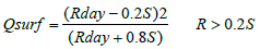 (1)
(1)
Where,
Qsurf is the accumulated run-off or rainfall excess (mm), Rday the rainfall depth for the day (mm), S is retention parameter (mm). Run-off will occur when Rday > 0.2S.
The retention parameter varies spatially due to changes in soil, land use, management and slope and temporally due to changes in soil water content. The retention parameter is defined as
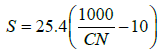 (2)
(2)
Where, CN is the curve number for the day
SWAT model set up
The SWAT model requires input parameters including a digital elevation model for contour and slope, climate, soil characteristics and land cover [16-18] (Figure 4). Additional information about water infrastructure and land management practices can also be incorporated. The first step in model construction is the delineation of the watershed and its associated sub-basins and reaches. As a physically based model, SWAT derives topography, contour and slope from a digital elevation model used to divide the basin into sub-watersheds.

Figure 4: Shows flow chart of SWAT model network.
Once the DEM is added, the model then uses the contours and watershed slope, calculated during the delineation, to determine flow direction and accumulation. Once flow direction and accumulation have been established, the model generates a stream network in which each individual reach drains a sub basin, all of which drain into a major reach. Each reach has a node or outlet. The modeller then selects a node that corresponds to the outlet at which the discharge measurements for calibration are being collected. This outlet sets the lower bound for the watershed basin, which is then delineated based on the location of that outlet and the stream network.
In order to define HRUs, the model requires data on land use, soil type and slope. Once land use, soil type and slope were defined, HRUs, were created with unique combinations of those classes. HRUs are the Hydrological response unit that divides the watershed into various homogeneous units based on the land use, soil type, and slope at each grid. Hydrologic response units for each sub basin were created. SWAT requires land use and soil data to determine the HRUs for each sub-basin. The land use and soil map have been imported in the model. Land use category is used to specify the land use layer and soil look up table is used to specify the type of soil to be modelled for each category in the soil layer, linked to the SWAT database and reclassified land use and soil map.
The soil map reclassified the database in 4 hydrological soil group (HSG) named A, B, C, D based on their infiltration rate. The land use, soil and slope maps were overlaid. Eliminate minor land use, soil and slope, threshold percentage method was adopted and 5% threshold for land use, 10% threshold for both soil and slope were used. The HRUs were delineated and corresponding report was also generated by the model which specified the area of different HRUs in various sub-basins.
The final step before simulation was the creation of input tables, including weather information. The weather data includes precipitation, maximum and minimum temperature, relative humidity, solar radiation and wind speed. Precipitation and temperature data are acquired from IMD. Relative humidity, solar radiation and wind speed data are collected from National Centers for Environmental Prediction (NCEP). These input file were set up and edited as per the requirement.
The watershed parameters showing the characteristics of surface runoff was defined. The files were successfully rewritten and stored in personal geo database of the model. After this step, the model was run to simulate the surface runoff.
Results and Discussions
The SWAT model has been run for the current study and output was generated at daily and monthly time step.
Hydrological modeling of Musi river basin using SWAT
During the watershed delineation the swat generates 21 sub basins. HRUs are generated by using land use and soil data. A total number of 152 HRUs were generated. Running the model the parameters have been edited according to the study area. The database has been rewritten doing necessary editing.
On successful run of the swat model, the accuracy of the result has been checked through swat check option. Manual calibration has been done for the errors shown in swat check. In this study area, runoff-rainfall ratio is found to be 0.3 for the time period 2008-2013. Surface runoff calculated by SWAT is 210.35 mm for a total rainfall of 818 mm. Evapo-transpiration for the study area is 529 mm for the same time period.
In this study, it is evaluated the relative sensitivity values found in the parameter estimation process. Sixteen parameters were found to be sensitive but the most sensitive parameters are eleven. To minimize as much uncertainty as much in the model results, the following parameters were changed during calibration: V_REVAPMN.gw, V_ SLSUBBSN.hru, V_SURLAG.bsn,R_CH_K2.Rte, R_GW_REVAP. gw, V_ESCO.hru, V_HRU_SLP_hru, V_GW_DELAY.gw, V_ ALPHA_BF.gw,V_GWQMN.gw and R_CN2.mgt. The description of stream flow calibration parameters are given in Table 1.
| Event Year | Cumulative Discharge in Cumecs | |
|---|---|---|
| Observed Qobs | Calculated by SWAT qsim | |
| 2010 | 9436.8 | 10374.24 |
| 2011 | 5874.7 | 4952.53 |
| 2013 | 18896.7 | 35648.49 |
Table 1: Observed versus Calculated year wise 2010, 2011 and 2013 cumulative discharges of Musi River Basin.
Comparative study has also been carried out for Musi river basin using SWAT model for the years 2010, 2011, and 2013. Preliminary analysis was tested with land use, soil, and weather data. The weather data includes precipitation, maximum and minimum temperature, relative humidity, solar radiation, and wind speed. This leads to 21 sub basins in the Musi river basin which is further sub divided into hydrological response units. The overall performance of the model in terms of NSE has been carried out using SWAT CUP. The observed and simulated outputs show satisfactory results. Hydrographs generated from the SWAT model are shown in Figures 5-7 respectively for the years 2010, 2011, and 2013. Table 1 indicates the cumulative discharges year wise i.e. 2010, 2011 and 2013 by simulation through SWAT model and observed data. Table 2 represents the observed and simulated peak discharges of Musi river basin from SWAT models for the years 2010, 2011, and 2013 at Damaracherla guage station.

Figure 5: Simulated and observed hydrographs at Damarcherla station from SWAT model for the year 2010.

Figure 6: Simulated and observed hydrographs at Damarcherla station from SWAT model for the year 2011.

Figure 7: Simulated and observed hydrographs at Damarcherla station from SWAT model for the year 2013.
| Year | Observed discharge (In Cumecs) | Simulated discharge (In Cumecs) by SWAT Model |
|---|---|---|
| 2010 | 461.5 | 516.3 |
| 2011 | 282 | 279.2 |
| 2013 | 3656.3 | 4386 |
Table 2: Observed and simulated peak discharges from the SWAT model.
SWAT model is a comprehensive conceptual model and relies on several parameters varying widely in space and time while transforming input into output. Calibration process becomes complex and computationally extensive when the number of parameters in a model is substantial. With the help of sensitivity analysis, reduce the number of parameters by not considering non-sensitive parameters for calibration, which in turn can give results relatively in short time. Sensitivity analysis is performed using the SUFI-2 algorithm of SWAT-CUP. The parameter producing the highest average percentage change in the objective function value is ranked as most sensitive.
SWAT Calibration and Uncertainty Program (SWAT-CUP) is a computer program which provides the calibration, validation and sensitivity analysis of SWAT models. It involves several methods such as SUFI2, PSO, GLUE, ParaSol, and MCMC which can be chosen for the purpose of calibration and uncertainty analysis. This accesses the SWAT input files and runs the SWAT simulations by modifying the given parameters.
The storage of the value of the objective function and the modification of parameters are the basis for comparison. Model calibration and validation is a challenging and to a certain degree subjective step in a complex hydrological model. The aim for the model simulation is to reflect natural conditions. Therefore, the SWAT model of Musi river basin was calibrated and validated using daily discharge available at Damarcherla. The simulation period was from 2008 to 2013 Table 3.
| Parameter name | Parameter description |
|---|---|
| A__GWQMN.gw | Treshold depth of water in the shallow aquifer required for return flow to occur (mm). |
| V__ALPHA_BF.gw | Baseflow alpha factor (days). |
| V__ESCO.hru | Soil evaporation compensation factor. |
| V__GW_DELAY.gw | Ground water delay in days |
| V__REVAPMN.gw | Threshold depth of water in the shallow aquifer for "revap" to occur (mm) |
| R__GW_REVAP.gw | Groundwater "revap" coefficient |
| R__CN2.mgt | SCS runoff curve number |
| R_CH_K2.rte | Effective hydraulic conductivity |
| V__SLSUBBSN.hru | Average slope steepness |
| V__HRU_SLP.hru | Average Slope length |
| V__SURLAG.bsn | Surface runoff lag coefficient |
Table 3: Stream flow parameters description.
The first two years were used as warm-up period to mitigate the effect of unknown initial conditions, which were subsequently excluded from the analysis. Based on the built-in sensitivity analysis tool in SWAT [19], identified the eleven most sensitive parameters and other parameters also being important for SWAT simulation in the Musi river basin. These 11stream flow calibration parameters are listed with fitted values in Table 4 as per daily basis and in Table 5 as per monthly basis.
| Parameter_Name | Fitted_Value | Min_value | Max_value |
|---|---|---|---|
| 1:R__CH_K2.rte | 0.016 | -0.2 | 0.2 |
| 2:V__ESCO.hru | 0.98 | 0 | 1 |
| 3:V__SLSUBBSN.hru | 40.799999 | 10 | 150 |
| 4:V__HRU_SLP.hru | 0.42 | 0 | 1 |
| 5:V__REVAPMN.gw | 10 | 0 | 500 |
| 6:R__GW_REVAP.gw | 0.16 | -0.2 | 0.2 |
| 7:V__SURLAG.bsn | 9.2 | 4 | 24 |
| 8:R__CN2.mgt | 0.12 | -0.2 | 0.2 |
| 9:V__ALPHA_BF.gw | 0.7 | 0 | 1 |
| 10:V__GW_DELAY.gw | 88.799995 | 30 | 450 |
| 11:V__GWQMN.gw | 300 | 0 | 3000 |
Table 4: Stream flow calibration parameters uncertainties on daily basis.
| Parameter_Name | Fitted_Value | Min_value | Max_value |
|---|---|---|---|
| 1:R__CH_K2.rte | -0.192 | -0.2 | 0.2 |
| 2:V__ESCO.hru | 0.62 | 0 | 1 |
| 3:V__SLSUBBSN.hru | 141.6 | 10 | 150 |
| 4:V__HRU_SLP.hru | 0.62 | 0 | 1 |
| 5:V__REVAPMN.gw | 290 | 0 | 500 |
| 6:R__GW_REVAP.gw | -0.192 | -0.2 | 0.2 |
| 7:V__SURLAG.bsn | 12.4 | 4 | 24 |
| 8:R__CN2.mgt | 0.032 | -0.2 | 0.2 |
| 9:V__ALPHA_BF.gw | 0.14 | 0 | 1 |
| 10:V__GW_DELAY.gw | 55.2 | 30 | 450 |
| 11:V__GWQMN.gw | 2700 | 0 | 3000 |
Table 5: Stream flow calibration parameters uncertainties on Monthly basis.
Based on stream flow uncertainty analysis in Table 4 fitted values with respects to minimum and maximum values on daily bases and in Table 5 on monthly basis are placed below. The distribution of sampling and parameter sensitivity on monthly time step are shown in Figure 8.

Figure 8: Plots showing most identified sensitive parameters during monthly calibration in SUFI2.
These parameters were considered for model calibration. The remaining parameters had no significant effect on stream flow simulations. The calibration process using SUFI-2 algorithm gave the final fitted parameters which are shown in above table for the basin. These final fitted parameter values were incorporated into the SWAT model for further applications. The fit between the model discharge predictions and the observed discharge showed good agreement as indicated by acceptable values of the NSE=0.71 and 0.70 for calibration period and 0.72 for validation period.
Calibration of the model
Calibration of the SWAT output is performed by using SWATCUP (SWAT Calibration and Uncertainty Procedures). In this an algorithm called SUFI (Sequential Uncertainty Fitting) is used for calibrating SWAT output with observed discharge. In SUFI-2, uncertainty of input parameters is depicted as a uniform distribution, while model output uncertainty is quantified at the 95% prediction uncertainty (95PPU). Sensitivity analysis was performed to identify which model Parameters had the greatest impact on surface runoff. Figure 8 plots showing most identified sensitive parameters during the monthly calibration in SUFI 2. The Table 6 represents the most sensitive parameters which are in order of ranking 1 to 11 based on P-value and T-Stat on daily basis and Table 7 indicates on monthly basis. After the sensitivity analysis, the model was calibrated using stream discharge data.
| Parameter | Ranking | T-stat | P-value |
|---|---|---|---|
| V_REVAPMN.gw | 11 | 0.3531558 | 0.7300974 |
| V_SLSUBBSN.hru | 10 | 0.63212779 | 0.5391606 |
| V_SURLAG.bsn | 9 | -0.7005385 | 0.4969498 |
| R_CH_K2. rte | 8 | 0.84494265 | 0.414672 |
| R_GW_REVAP.gw | 7 | 0.93344574 | 0.3689923 |
| V_ESCO.hru | 6 | 1.10505755 | 0.2907989 |
| V_HRU_SLP_hru | 5 | -1.4538136 | 0.1716473 |
| V_GW_DELAY.gw | 4 | 2.29156537 | 0.0408158 |
| V_ALPHA_BF.gw | 3 | -2.5947358 | 0.0234523 |
| V_GWQMN.gw | 2 | 3.24026838 | 0.0070831 |
| R_CN2.mgt | 1 | -8.484715 | 2.049E-06 |
Table 6: Parameters Sensitivity for SUFI-2 on daily basis.
| Parameter | Ranking | T-stat | P-value |
|---|---|---|---|
| V_HRU_SLP_hru | 11 | 0.042389227 | 0.966832 |
| V_GW_REVAP.gw | 10 | 0.238629401 | 0.815113 |
| V_ESCO.hru | 9 | 0.400196911 | 0.695510 |
| V_SURLAG.bsn | 8 | -0.459525418 | 0.653447 |
| V_REVAPMN.gw | 7 | 0.625828410 | 0.542259 |
| V_GW_DELAY.gw | 6 | -0.963711909 | 0.352775 |
| R_CH_K2. Rte | 5 | 1.291671752 | 0.218963 |
| V_GWQMN.gw | 4 | 1.595398915 | 0.134635 |
| V_ALPHA_BF.gw | 3 | -1.850432380 | 0.087103 |
| V_SLSUBBSN.hru | 2 | -2.155143678 | 0.050479 |
| R_CN2.mgt | 1 | -4.106147074 | 0.001238 |
Table 7: Parameters sensitivities for SUFI-2 on monthly basis.
It is noted from sensitivity analysis, parameters which are mostly responsible for the model calibration and parameter changes during the model iteration process. The remaining parameters had no significant effect on stream flow simulations. In SUFI-2 during daily calibrations Curve Number, threshold depth of water in shallow aquifer required for return flow, base flow alpha factor and ground water delay time have shown large distribution in their values. However in monthly calibrations Curve number, Average Slope steepness, in addition to the threshold depth of water in shallow aquifer required for return flow, base flow alpha factor and ground water delay time have shown large distribution in their values.
Evaluation of the model performance
The performance of SWAT model is analyzed based on graphical representation of observed and simulated total flow and observed and simulated sediment yield as well as on the basis of various statistical parameters such as. Using model outputs, Nash Sutcliffe efficiency (NSE) statistical index was generated to assess the accuracy of the model. An NSE of zero or less indicates the simulation is not able to predict discharge while an NSE of 1 indicates the model’s performance falls within an acceptable range of uncertainty Nash Sutcliff Efficiency (NSE) , Percent bias (Pbias), and RMSE-observations Standard deviation Ratio (RSR).
To evaluate the performance of the developed SWAT model quantitatively, statistical analysis the Nash–Sutcliffe model efficiency coefficient is used to assess the predictive power of hydrological models. It is defined as below:
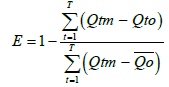 (3)
(3)
Where
Qtm is modelled discharge at t time, Qto is observed discharge at time and Qo is mean observed data at t time period
Nash–Sutcliffe efficiency can range from −∞ to 1. An efficiency (E) = 1 represents to a perfect match of modeled discharge to the observed data. An efficiency (E) = 0 represents that the model predictions are as accurate as the mean of the observed data, whereas an efficiency (E) <0 occurs when the observed mean is a better predictor than the model or, in other words.
Pbias or percentage of deviation measures the average tendency of the simulated values to be larger or smaller than the observed values.
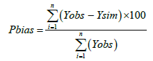 (4)
(4)
The optimal value of Pbias is 0 with low magnitude values indicating accurate model simulation. Positive values indicate model under estimation bias and negative values indicate model over estimation bias. RMSE-observations Standard deviation Ratio (RSR) standardizes the Root Mean square error using observations standard deviation. RSR is calculated as the ratio of RMSE and standard deviation of measured data as shown below
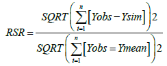 (5)
(5)
RSR varies from the optimal value of 0 to large positive value. 0 indicates zero residual variation and therefore perfect model. General performance rating for acceptable statistics is given in Table 8 for a monthly time step. Table 9 shows the performance rating of SWAT model statistics on monthly time step and simulated values are correlates with very good rating of stream flow.
| Performance rating | RSR | NSE | Pbias (%) | |
|---|---|---|---|---|
| Stream flow | Flow Sediment | |||
| Very good | 0.00 to 0.50 | 0.75 to 1.00 | < ± 10 | < ± 15 |
| Good | 0.50 to 0.60 | 0.65 to 0.75 | ± 10 to ± 15 | ± 15 to ± 30 |
| Satisfactory | 0.60 to 0.70 | 0.50 to 0.65 | ± 15 to ± 25 | ± 30 to ± 55 |
| Unsatisfactory | > 0.70 | < 0.50 | > ± 25 | > ± 55 |
Table 8: General performance ratings for recommended statistics for a monthly time step.
| Pbias | NSE | RSR |
|---|---|---|
| Calibration period | ||
| -2.75 | 0.71 | 0.12 |
| -1.26 | 0.70 | 0.12 |
| Validation period | ||
| -4.55 | 0.72 | 0.20 |
Table 9: Performance rating of the SWAT model Statistics ( monthly basis).
Discussion
Musi River watershed delineation the SWAT generates 21 sub basins. After that HRUs are generated by using land use and soil data. A total number of 152 HRUs were generated. It is observed that most of the basin has general smooth slope, especially near the river origin falls under steep slopes. This high altitude area contributes to a significant amount of soil erosion and as well as high run off. Clay, clay skeletal, loamy and loamy skeletal soils are the most dominating soil categories found in this Musi river basin.
The average annual flow for daily basis of the time series computed for calibration period years 2010 &2011 are 66.93 and 31.95 Cumecs against observed average annual flow 60.88 Cumecs and 37.90 Cumecs. The average annual flow of the time series computed for validation period year 2013 is 229.99 Cumecs and observed average annual flow is 121.99 Cumecs. The time –series data of the observed and simulated flows on daily and monthly basis for the period from 2010 to 2013 were plotted hydrographs of simulated match well with validated hydrograph.
Conclusion
With this hydrological modeling approach, the simulation indicates that the computed hydrographs match well with the observed hydrographs. Accuracy in computing peak discharge was 75 percent approximately when compared to the observed flows. After considering the uncertainties during model inputs and parameterization the SWAT model gave good simulation results for daily and monthly time series for Musi river basin.
The performance of the model for runoff estimation on daily basis for calibration & validation period statistics found to be good as per Nash–Sutcliffe model efficiency coefficient for calibration period with 0.71 and validation period with 0.72. The absolute percentage error for monthly basis for calibration &Validation period statistics are (Pbias) less than +/- 10% (i.e., -2.75, -1.26 for calibration period and -4.55 for validation period.) found to be stream flow is reasonably well and RMSE-observations standard deviation ratio (RSR) value calculated for calibration 0.12 and validation period 0.20 which are <0.5 and found to be stream flow is reasonably well.
The hydrological water balance analysis using SWAT model indicates excessive runoff due to high curve number value. The base flow and percolation are notified as important components and responsible for total discharge at the given out let i.e. at Damarcherla gauge station of the study area more than 33% of the loses in the watershed are found through evapotranspiration. The alpha factor is a direct index of the intensity with which groundwater outflow responds to changes in recharge. As the alpha level was increased, the deviation between observed and simulated discharge increased.
After considering the all uncertainties during the model inputs and parameterization, SWAT model gave good simulation results for daily and very good simulation results monthly time series for Musi river basin. However, this whole model uncertainty and calibration analysis can be used for futuristic prediction and assessment of water balance and climate change studies as well as other management scenarios for stream flow measurements especially for the Musi River basin.
References
- Jain M, Sharma SD (2014) Hydrological modeling of Vamshadara River Basin, India using SWAT. International Conference on Emerging Trends in Computer and Image Processing (ICETCIP-2014), Pattaya, Thailand.
- Simić Z (2009) SWAT-based runoff modeling in complex catchment areas theoretical background and numerical. Journal of the Serbian Society for Computational Mechanics 3: 38-63.
- Nerella S (2000) Improvement of domestic waste water quality by subsurface flow constructed wetlands. Bioresource Technology 75: 19.
- Neitsch SL (2009) Soil and water assessment tool input/output file documentation. College Station. TX: Texas Water Resources Institute.
- Easton ZM (2008) Re-conceptualizing the soil and water assessment tool (SWAT) model to predict runoff from variable source areas. Journal of Hydrology 348: 279-291.
- White ED (2011) Development and application of a physically based landscape water balance in the SWAT model. Hydrological Processes 25: 915-925.
- Arnold JG (1998) Large area hydrologic modeling and assessment, part I: model development. Journal of American Water Resources Association 34:73-81.
- Kannan N, White SM, Worrall F, Whelan MJ (2007) Sensitivity analysis and identification of the best evapotranspiration and runoff options for hydrological modeling in SWAT-2000. J Hydrol 332: 456-466.
- Pandey A (2008) Runoff and sediment yield modeling from a small agricultural watershed in India using The WEPP model. Journal of Hydrology 348: 305-319.
- Tripathi MP, Panda RK, Raghuwanshi NS (1999) Estimation of sediment yield from a small watershed Using SWAT model. Asian Institute of Technology 87-96.
- Singh A, Imtiyaz M (2012) Application of process based hydrological model for simulating stream flow in an agricultural water shed of India. India Water Week 2012- Water Energy and Food Security Call for Solutions, New Delhi, India.
- Setegn SG, Srinivasan R, Dargahi B (2008) Hydrological modelling in the Lake Tana Basin, Ethiopia using SWAT model. Open Hydrol J 2: 49-62.
- Yang J, Reichert P, Abbaspour KC, Xia J, Yang H, (2008) Comparing uncertainty analysis techniques for a SWAT application to the Chaohe Basin in China. J Hydrol 358: 1-23.
- Singh V, Bankar N, Salunkhe SS, Bera AK, Sharma JR (2013) Hydrological stream flow modeling on tungabhadra catchment: parameterization and uncertainty analysis. Current Science 104: 1187-1199.
- Arnold JG, Allen PM, Muttiah R, Bernhardt G (1995) Automated base flow separation and recession analysis techniques. Ground Water 33: 1010-1018.
- Monteith JL (1965) Evaporation and environment. Proc SympSoc Exp Biol 19: 205-234.
- Willams J (1969) Flood routing with variable travel time or variable storage coefficients. Trans ASAE 12: 100-103.
- Arnold JG, Kiniry JR, Srinivasan R, Williams JR, Haney EB, et al. (2012) Soil and water asssessment tool input/output documentation. TR-439, Texas Water Resources Institute, College Station, 1-650.