Research Article, Res Rep Math Vol: 1 Issue: 1

Meromorphic Functions and Theta Functions on Riemann Surfaces

Lesfari A^*

Department of Mathematics, Faculty of Sciences, University of Chouaib Doukkali, Morocco

*Corresponding Author : Lesfari A
Department of Mathematics, Faculty of Sciences, University of Chouaib Doukkali, B.P. 20, 24000 El Jadida, Morocco
Tel: +212 5233- 44448
E-mail: lesfariahmed@yahoo.fr

Received: August 01, 2017 Accepted: August 20, 2017 Published: August 28, 2017

Citation: Lesfari A (2017) Meromorphic Functions and Theta Functions on Riemann Surfaces. Res Rep Math 1:1.

Abstract

Keywords: Riemann surfaces; Meromorphic functions; Theta functions

Introduction

Let X be a compact Riemann surface of genus g ≥1 and a square matrix of order g, symmetric and Im B > 0. We consider the Riemann theta function θ(z|B) defined by its Fourier series:

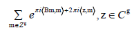(1)

Where

The convergence of this series for all results from the fact that Im B >0. We show that this series converges absolutely and uniformly on compact sets and thus the function θ(z|B) is holomorphic over C^g.

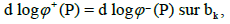
When the matrix B is fixed, we will put in the sequel .Let (e₁, ..., e_g) be a basis of with and let be the columns of the matrix B or in condensed form f_j = b_ej, j=1, ..., g.

Theorem 1

The function θ satisfies the functional equations

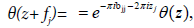(2)

For any we have

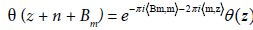(3)

Any vectors of the form n + B_m is a period of the Riemann theta function, they constitute the period lattice.

Proof: The first relation results from formula (1). Concerning the second relation, we have

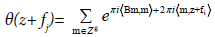
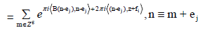
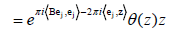
And, the relation (3) immediately follows.

Thus the vectors e₁,..., e_g are the periods of function θ(z). The vectors f₁,..., f_g are called the quasi-periods. The function θ is quasiperiodic and is well defined on the Jacobian variety of X.

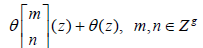
Consider a generalization of the theta function (1) called the theta function with characteristics α and β

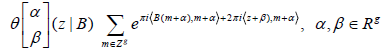(4)

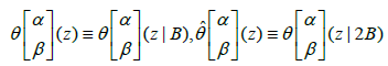
To simplify the formulas, we simply note:

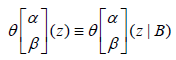
when the matrix B is fixed. In particular,

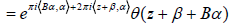
From equation (3), we have also

Consequently, it is sufficient to consider the functions where 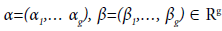are such that: 0 < α_j, β₁< 1, j = 1, ..., g.

Theorem 2

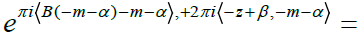
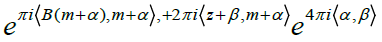
The periodicity property of the theta-functions with characteristics is given by the following relation.

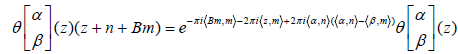
Proof

It suffices to reason as in the previous proposition.

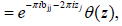
If α₁,… α_g and β₁,…, β_g a are 0 or , we will say that the set is a half period. In addition, a half period is said to be even if 4 (α, β) ≡ 0 (mod. 2) and odd if not.

Theorem 3

The function is even if half-period (z) is even and odd if half-period is odd. In addition, we have θ(z)=θ(-z).

Proof: By making the substitution

z →−z, m →−m − 2,

into (4), we obtain immediately for the general term of the series,

Now, from the above definition, the sign is determined by the parity of the number 4 (α, β), and the last relation results.

For example, the number of even half-periods is equal to 2^g−1 (2^g + 1) and of odd half-periods to 2^g−1(2^{g − 1}).

Meromorphic Functions Expressed in Terms of Theta Functions

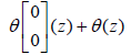
Consider the case of Riemann surfaces of genus 1, i.e., elliptic curves. Let us recall that an elliptic function is a doubly periodic meromorphic function. In this case, the matrix B is reduced to a number that we denote by b with Im b≥0. The numbers 1 and b generate a parallelogram of the periods denoted Ω. The four theta functions corresponding to the half-periods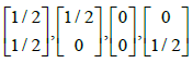 are.

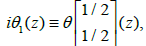
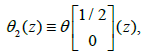
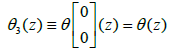
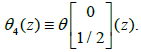
These functions are holomorphic on. Moreover, we immediately deduce from theorem 3 thatθ₁(z) is odd and thatθ₂(z), θ₃(z), θ₄(z), are even. To determine the zeros of the functions θj it is sufficient, from theorem 2, to look for them in the parallelogram of the periodsΩ. Sinceθ₁(z) is odd, thenθ₁(0)=0 and the other zeros of θ_j(z) are obtained via theorem 2. In particular we see that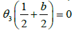 . We claim that this zero of θ₃(z), in

Ω is unique, which is easy to prove. Namely, we need to prove that along boundary δΩ.

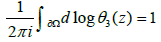
We have

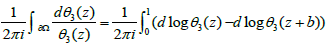
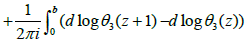
From theorem 2, we have

So

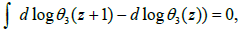
And

Therefore

and we have the following result:

Theorem 4

The function θ(z) has in the parallelogram of the periods Ω generated by 1 and b), only one zero at the point

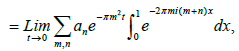
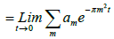
By putting z = x ∈ R, b = it, t ∈ R+, we shall see (following [16]) θ (x|it) as the fondamental periodic solution to the heat equation. Equation (1) is written

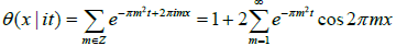
Thus θ is a real valued function of two real variables. This function is periodic with respect to x, i.e., θ(x+1|it)=θ (x|it). Since

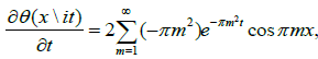
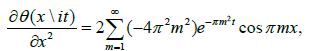
Then

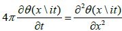
This suggests that we characterise the theta function θ(x|it) as the unique solution to the heat equation with a certain periodic initial data when t=0. To examine the limiting behaviour of f, we integrate it against a test periodic function

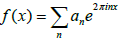
Then

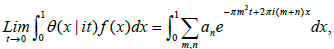
=f(0)

Hence θ(x|it) converges, as a distribution, to the sum of the delta functions at all integral points x∈ Z as t→0. The uniqueness of this solution results from the fact that

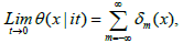
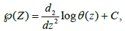
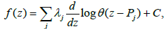
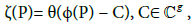
Where δ_m is the distribution of Dirac at m. We have previously studied the convergence of the theta function. Thus θ(x|it) may be seen as the fundamental solution to the heat equation when the space variable x lies on a circle R/Z. Similarly, the function θ1(z) satisfies a third-order differential equation. Indeed, it is enough to use the relation.

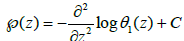
where C is a constant is the Weierstrass function defined by

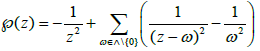
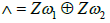is the lattice generated by two non-zero complex numbers ω₁ and ω₂ such that: , and take into account the differential equation:

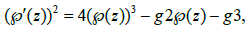(6)

Where

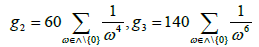
Moreover, we have the following classical identities [1-16]:

Theorem 5

The theta function satisfies the addition formulas.

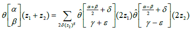
where

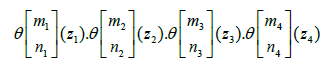
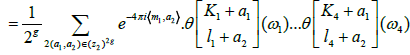
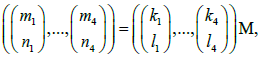
where (z₁, ..., z₄) = (w₁, ...,w₄)M with

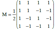
Here 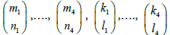are arbitrary vectors of order 2g with

and 1 denotes the unit matrix of order g or 2g.

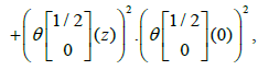
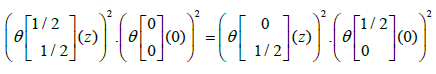
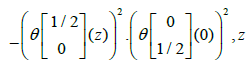
In particular, we have the formulas:

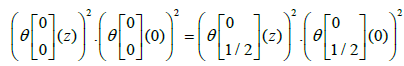
And

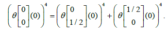
as well as the identity of Jacobi obtained by posing z = 0,

We shall see how to express the meromorphic functions on the torus C/Λ in terms of the theta function. Several approaches are possible:

Approach 1

Recall that any rational fraction (hence a meromorphic function on P¹(C)) can be written in the form

(7)

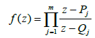
By analogy, let P₁, ..., P_m,Q₁, ...,Q_m be points of the Riemann surface X and f(z) a function having zeros at the points P₁, ..., P_m and poles at points Q₁, ...,Q_m. It is assumed that condition (i) (or what is equivalent, condition (ii)) of Abel’s theorem1 is satisfied. Since X has genus 1, then there exists a single holomorphic differential ω on X. Still according to Abel’s theorem [1], the existence of the function f(z) imposes the condition.

P₁ + P₂ + · · · + P_m = Q₁ + Q₂ + · · · + Q_m

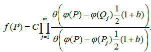
Note that for m = 1; P₁ = Q₁ and the only valid case is f(z)=constante. In the case where m≥2, the function f(z) may be expressed in terms of θ as follows:

(8)

where C is a constant. This formula may be considered as the straightforward generalization of the representation (7) for the meromorphic (rational) function on P1(C). The most important difference is that in (7) the positions of the poles and zeros are arbitrary. To verify that f(z) in (8) is indeed single valued on X we have to check that f(z + 1) = f(z) and f(z + b) = f(z).

The first relation is trivial and according to relation (2) and the fact that 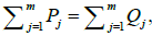we also have the second relation. Thus f is doubly periodic. The function f is meromorphic with zeros in and poles in

Approach 2

The function log θ(z) can be expressed as the sum of a doubly periodic function of periods 1, b and a linear function. Therefore the function is doubly periodic and meromorphic over X, with a double pole in . This function coincides with the Weierstrass function :

(9)

Where C is a constant chosen in such a way that Laurent’s series expansion of en Z=0 has no constant term. The connection given by (9) between the Weierstrass function and the theta function is obvious in view of

the right-hand side (as noted above) and the information obtained above on the location of the zeros of θ(z). Now from (9) and (6) it follows that the function (z) satises a dierential equation of 3^rd order.

Approach 3

Recall that meromorphic functions with simple poles on P₁(C) can be written in the form

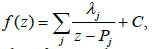
where λ_j∈C and C is a constant. By analogy, we consider on X the function

where P_j∈X, λ_j∈C such that Σ_jλ_j=0 et C is a constant. This function is doubly periodic and meromorphic with simple poles in and residues λ_j at these points.

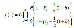
We have seen how the meromorphic functions on the torus C/Λ can be expressed in terms of theta function. Moreover, for g=1, we know that: 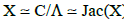. So the construction that was done previously on the torus C/Λ or what amounts to the same on Jac(X) is also valid on the Riemann surface X. For example, let us take the case of a function having poles in P₁,..., P_m and zeros in Q₁, ...,Q_m on the Riemann surface X. According to Abel’s theorem, we have

and it is possible, according to approach 1 described above, to express the function f(P) in terms of theta function using the formula

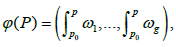
Let us now pass to the case where the surface of Riemann X is of genus g>1. Recall that the Jacobi inversion problem [5,16] consists in determining g points P₁, ..., P_g on X such that:

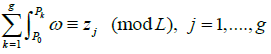
Where (z₁, ..., z_g) ∈ Jac(X), (ω₁,…,ω_g) is a base of holomorphic differentials on X, P₀ is a base point on X and L is a lattice generated by the column vectors of the period matrix. In other words, the problem is to determine the divisor in terms of z = (z₁, ..., z_g) 2 Jac(X) such that if ‘ is the Abel-Jacobi map, then the equation Ï�? (D) = Z is satisfied. We will study the Jacobi inversion problem using theta functions.

Theorem 6

If the function defined by

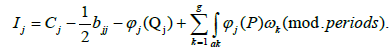
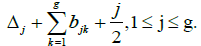
is not identically zero, then it admits g zeros (counted with their order of multiplicity) on the normal representation X* of X, denoted by the symbol 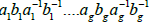, where (a₁, . . . , a_g, b₁, . . . , b_g) Is a symplectic basis of the homology group H₁(X, Z). Moreover, if P₁, ..., Pg denote the zeros of this function then we have on the Jacobian variety Jac(X) the formula.

(mod. periods)

Where is the vector of the Riemann constants defined by

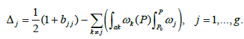(10)

Proof:

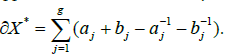
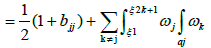
Note that X* is a polygon with 4g sides identified in pairs. If one traverses the boundary δX*of this polygon, we notice that each side is traversed twice, one in the direction of its orientation and the other in the opposite direction. So δX* may be represented as follows

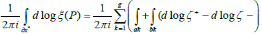
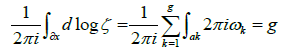
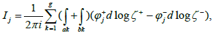
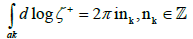
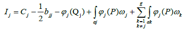
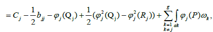
To calculate the number of zeros, we have to compute the integral (logarithmic residue): 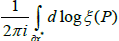We denote by ζ-the value of the function ζ(p) on and by ζ+ the value of ζ(p) on the segments aj,bj. We will use similar notations Ï�? + , Ï�? − for the Abel map Ï�? ( p) . In this notation the above integral can obviously be rewritten in the form

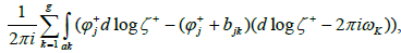
Note that

if P∈a_k and

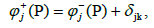
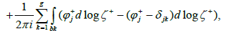
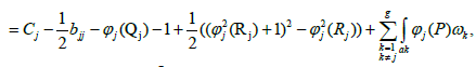
if P∈b_k. From Theorem 4, we have

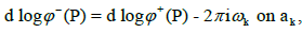
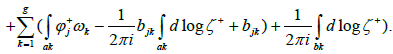
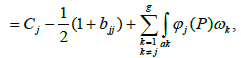
Therefore (2), implies

which shows that the function ζ(p) admits g zeros on X*. To prove the second part of the theorem, we consider the integral

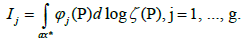
By designating P₁, ..., P_g the zeros of the function ζ(p) and taking into account the residual theorem, we have

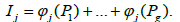
By reasoning as before, one obtains

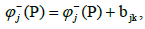
Note that

Similarly, by designating by Q_j (resp. Q^* _J ) the beginning (or end) of the contour bj, then

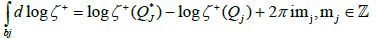
where 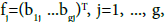denote the columns of the matrix B. Therefore,

The beginning of the contour aj will be designated by R_j and its end obviously, coincides with the beginning Q_j of the contour b_j. We have

which ends the proof.

In general, the vector Δ depends on P0 except in the particular case g = 1, Where = . We show that 2Δ=Ï�?−(K), where K is the canonical divisor. Hence, by skillfully choosing the point P₀ we can express K in a very simple way. For example, consider the case where X is a hyperelliptic curve of genus g of affine equation.

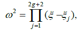
where all zj are distinct. Let (a₁, . . . , a_g, b₁, . . . , b_g) be a symplectic basis of the homology group H₁(X, Z)) and let

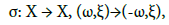
the hyperelliptic involution (i.e., which consists in exchanging the two sheets of the curve X) with (a_j) = −a_j and σ (b_j) = −b_j . Note that

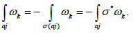
Then, by choosing we get

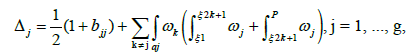
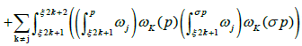
Taking into account that ω_k (σP)= ω_k (P) and modulo a linear combination n+B_m (a lattice generated by the column vectors of the period matrix), we obtain in this case the formula :

The zeros of a theta function on form a submanifold of Jac(X) of dimension g − 1 called theta divisor Θ={z : θ(z) = 0}. It is invariant by a finite number of translations and can be singular. Equation (3) implies that Θis well defined on the Jacobian variety Jac(X). Since θ(z) = θ(z), we deduce that Θ is symmetric: -Θ=Θ.

Theorem 7

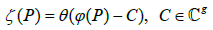
(Riemann). The function

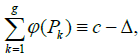
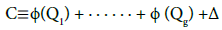
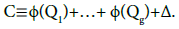
is either identically zero, or admits exactly g zeros Q₁, ...,Q_g on X such that:

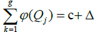
where Δ is defined by (10).

This result means that when we embed the Riemann surface X into its Jacobian variety Jac(X) via the Abel map Ï�?, then its image is fully include in the theta divisor, or it meets it in exactly g points. In fact, if ζ(P) is not identically zero on X, then its zeros coincide with the points P₁, ..., Pg and determine the solution of the Jacobi inversion problem Ï�?(D) = z for the vector z = C −. Recall that D ∈ Div(X) is a special divisor if and only if dim L(D)≥ and dim L(K −D) ≥1where K is a canonical divisor. In the

case where D ≥ 0 a divisor is special if and only if dim Ω1(D)≠0 Note also that the special divisors of the form

coincide with the critical points of the Abel-Jacobi map,

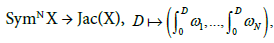
or what amounts to the same

These critical points are the points P1, ..., PN where the rank of the differential of this application is less than g. From Riemann’s theorem 7, the function ζ(P) = θ(Ï�? (P) − C) is identically zero if and only if

where Q₁ + · · · + Q_g is a special divisor.

Theorem 8

Let be a vector such that the function

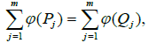
is not identically zero on X. Then the function ζ(P) admits exactly g zeros P₁, ..., P_g on X which determine the solution of the Jacobi inversion problem

where i.e., the solution of

(12)

(recall that the symbol≡, as usual, means congruence modulo the period lattice). Moreover, the divisor D is not special and the points P₁, ..., P_g are only determined from the system (12) up to a permutation.

Proof

The first assertion results from theorem 1. Moreover, the divisor is not special because otherwise the function ζ(P) would be identically null from what precedes, which is absurd. For the last point, assume that the system (12) admits another solution Q₁, ...,Q_g. We will have on the Jacobian variety Jac(X),

where L is the lattice generated by the period matrix. According to Abel’s theorem, this means that there exists a meromorphic function on X having zeros in Q₁, ...,Q_g and poles in P₁, ..., P_g. Now we have just shown that the divisor is non-special, so such a function must be a constant, which means that P_j = Q_j , j = 1, ..., g.

For example, if

is a non-special divisor on a Riemann surface X of genus g, then the function θ(Ï�?(P) – Ï�?(D)–Δ), admits exactly g zeros on X at the points P = P₁, ..., P_g. We have the following characterization of the theta divisor:

Theorem 9

We have θ(C) = 0, if and only if there exists with base point P0, such that:

Proof

Let us return to the function

and assume first that it is non-zero on X. By theorem 6, this function admits g zeros P₁, ..., P_g on X and

(13)

The set of these zeros being unique and as by hypothesis θ(C) = 0, then P_g = P₀. Therefore Ï�?(P_g)= Ï�?(P₀) and from (13), we have

Let us now turn to the case where the function ζ(P) is not identically zero on X. According to theorem 6, we have

(14)

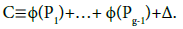
where Q₁ +· · ·+Q_g is a special divider. The latter implies the existence on X of a non-constant meromorphic function ζ having poles in Q₁, ...,Q_g with (P₀)=0. Then,

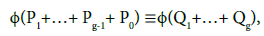
according to the Abel theorem where P1 + · · · + Pg−1 + P0 is the divisor of the zeros of ζIt is therefore suâ�?�?cient to replace in the formula (14), Ï�?(Q₁+…+ Q_g), by Ï�?(P₁+…+ P_g-1+ P₀) while taking into account that (P0) = 0.

Theorem 10

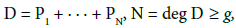
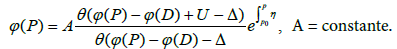
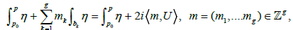
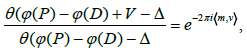
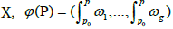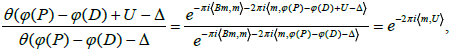
Let D be a non-special divisor of degree g, D′ a positive divisor of degree n, a positive divisor of degree n, (ω₁,…,ω_g) a base of holomorphic differentials on a base of holomorphic differentials on the Abel map with base point P0, η normalized differential of the 3^rd kind 2 on X having poles on D′ and residues −1, U = (U₁, ...,U_g) the vector-periods with and finally Δ the vector defined using the Riemann constants by (10). If ψ is a meromorphic function on X having g + n poles on D + D′, then this function is expressed in terms of theta function by the formula

Proof: It should be noted that the integration contour in integrals and 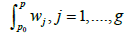is the same. The function ψ (P) admits poles only on D + D′. Let us show that this function is well defined on X; i.e., it does not depend on the path of integration. In other words, it does not change when P goes through any cycle 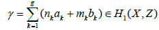the expressions and 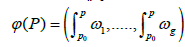is transformed respectively as follows:

and Moreover, using formula (4), one obtains

and the result follows from the above transformation.

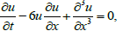
On the Riemann surface X of genus g, singular functions possessing g poles and essential singularities play a crucial role in the study of integrable systems, in particular the Korteweg-de Vries equation K-dV),

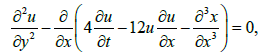
the Kadomtsev-Petviashvili equation (KP),

the nonlinear Schrödinger equation

the Boussinesq equation

the Camassa-Holm equation

whose exact solutions are solitons [14], i.e., self-reinforcing solitary waves that maintain their shape as they propagate at a constant rate. We shall see by analogy from the previous theorem how to express these functions (known as Baker-Akhiezer functions) in terms of theta functions and at the same time prove their existence. Let Q₁, ...,Q_n be points on a Riemann surface X of genus g and z_j are local parameters such that : z_j(Q_j) = ∞. We associate to each point Q_j an arbitrary polynomial denoted by q_j(z_j).

Let

be a positive divisor on X and ψ(P) a function (called Baker- Akhiezer function) satisfying the following conditions :

(i) ψ(P) is meromorphic on X\ {Q₁, ...,Q_n} and admits poles only at the points P₁, ..., P_n of the divisor D.

(ii) the function is analytic in the neighbourhood of Qj ,j=1, ..., n.

The condition (ii) can be replaced by this condition: the function ψ admits an essential singularity of the form at the points Q_j, j = 1, ..., n where c is a constant. These functions ψ(P) form a vector space that we note L≡ L(D;Q₁, ...,Q_n, q₁, ..., q_n).

Theorem 11

Let D = P₁ + · · · + P_g be a non-special divisor of degree g. Then the space L is of dimension 1 and its basis is described using

(15)

Where ηis a normalized differential of the 2^nd kind³ having poles at the points Q₁, ...,Q_n, the main parts coincide with the polynomials q_j(z_j), where j = 1, ..., n, V = (V₁, ..., V_g) with V_k=

the Abel map with base point P₀, Δ is the vector defined using the Riemann constants by (10). The integration contour in integrals and 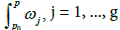is the same.

Proof: The function ψ₁(P) has poles on the divisor D and essential singularities at the points Q₁, ...,Q_n. The function ψ₁(P) is well defined; It does not depend on the integration path. Using the notations and reasoning similar to those of theorem 10, we obtain

and the result follows from the transformation used in the proof of the preceding theorem. Moreover, according to the Riemann- Rock theorem [5,15], the dimension of the space L is equal to deg D−g+1. As deg D=g, then the dimension of the space in question is equal to 1, which proves the uniqueness of the function with ψ₁ (to a multiplicative constant). Let ψ₁ ∈L be any function. Therefore, the quotient is a meromorphic function with g(= degD) poles. The divider of the poles of coincides with the divisor 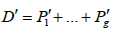of the zeros of

and we must have Ï�?(D′)-Ï�?(D)=Vy choosing the polynomials qj with sufficiently small coefficients (or what amounts to the same, the vectors of V sufficiently small), then the theta function which is in the numerator of the above expression is not identically zero. Therefore, its divisor D′ of the poles is not special and therefore is a constant.

Examples

It is well known that the solutions of many integrable systems are given in terms of theta functions associated with compact Riemann surfaces. We will see below some solutions for some interesting problems.

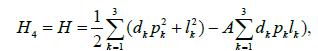
As a first example, we consider the motion of a solid in a perfect fluid described using the Kirchhoff equations [3]:

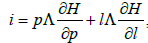
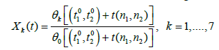
Where, and H is the Hamiltonian. This system has the following three first integrals:

H₁=H,

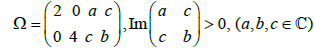
Two cases can be distinguished: case of Clebsch and case of Lyapunov- Steklov. In the case of Clebsch,

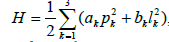
with condition

The above system is written in the form of a Hamiltonian vector field. A fourth first integral is given by

where is a constant such that

The method of resolution obtained by Kötter [9] is extremely complicated and relies on an astute choice of two variables s1 and s2. Using the substitution , and an appropriate linear combination of H1 and H2, we can rewrite the above equations in the form

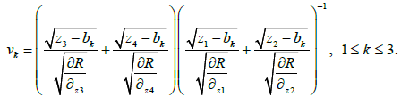
where A, B, C et D are constants. Let us introduce coordinates Ï�?_k, ψ_k, 1≤k≤3 by setting

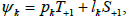
and

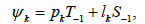
where

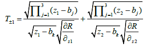
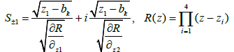
and z₁, z₂, z₃, z₄ are the roots of equation

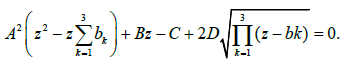
Let s₁ and s₂ be the roots of equation

Where

We can express the variables p₁, p₂, p₃, l₁, l₂, l₃ in terms of s₁ and s ₂ [9]. After some algebraic manipulations, we obtain

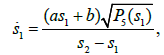
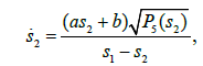
where a, b are constants and P₅(s) is a polynomial of degree five having the following form:

Consequently, the integration is done by means of hyperelliptic functions of genus 2 and the solutions can be expressed in terms of theta functions. The problem of this motion is a limit case of the geodesic flow on SO(4). Let us remind that for an algebraically completely integrable system [1], we require that the invariants of the deferential system be polynomial (in appropriate coordinates) and that the complex manifolds obtained by equating these polynomial invariants with generic constants form the afine part of a complex algebraic torus (Abelian variety) in such a way that the complex flow generated by the invariants are linear on these complex tori. Meromorphic solutions dependent on a sufficient number of free parameters play a crucial role in the study of these systems. We show [1,6] that the differential system.

in question is algebraically completely integrable and the corresponding flow evolves on an Abelian surface

where the lattice is generated by the period matrix.

The affine surface M_c defined by putting the invariants of the system equal to generic constants, can be completed into a nonsingular compact complex algebraic variety (Abelian surface) 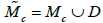by adjoining at in infinity a smooth curve D of genus 9. The latter is a double cover of an elliptic curve ε ramified over 16 points. The application

is an embedding of into where (1,X₁, ...,X₇) forms a base of the space L(D) of meromorphic functions with at worst a simple pole along D (The functions X₁, ...,X₇ are expressed in a simple way as a function of x₁, ..., x₆). The solutions of the differential system in question in terms of theta functions are given by

where (θ₀, ..., θ₇) forms a base of the space of theta functions associated with D. The two functions theta θ_{0, 7} are odd while the six functions theta θ₁, ..., θ₆ are even. In the case of Lyapunov-Steklov,

where A, B and C are constants. A fourth first integral is given by

where A long and delicate calculation [10] shows that in this case too, the integration is performed using hyperelliptic functions of genus two and the solutions can be expressed in terms of theta functions. Another interesting example concerns the Landau-Lifshitz equation [2,11]:

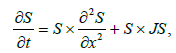
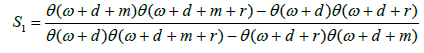
where 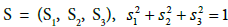and J=diag (J₁, J₂, J₃). This equation describes the effects of a magnetic field on ferromagnetic materials. The real solutions (with magnetic anisotropy of the axis of easy magnetization type) are given by

Here the theta function is linked to a hyperelliptic curve of genus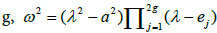 whose cycle encircles the cut [1a,a], where the integration path crosses the cycle the vector is such that : Im

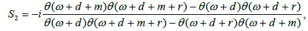
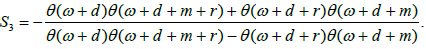
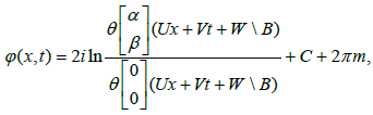
We cite yet another example which concerns the sine-Gordon equation [2]:

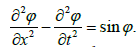
It is a non-linear wave equation with multiple applications in physics. Its solution can be written in the form

Moreover, the study of the theta functions of a Riemann surface of the genus g can be done from the point of view of tau function of a hierarchy of soliton equations [13]. The tau functions are specific functions of time, constructed from sections of a determinant bundle on a Grassmannian manifold of in definite dimension and generalize the Riemann theta functions.

References

1. Adler M, van Moerbeke P, Vanhaecke (2004) Algebraic integrability, Painlevé geometry and Lie algebras, Springer-Verlag, New York, USA.
2. Belokolos AI, Bobenko VZ, Enol'skii VZ, Its AR, Matveev VB (1994) Algebro-Geometric approach to nonlinear integrable equations. Springer-Verlag, New York, USA.
3. Dubrovin BA (1981) Theta functions and non-linear equations. Russ Math Surv 36: 11-92.
4. Fay JD (1973) Theta functions on Riemann surfaces. Lecture notes in mathematics, Springer-Verlag, New York, USA.
5. Griffiths P, Harris J (1978) Principles of algebraic geometry. Wiley-Interscience, USA.
6. Haine L (1983) Geodesic flow on So(4) and Abelian surfaces. Math Ann 263: 435-472.
7. Igusa JI (1972) Theta-functions. Springer Berlin Heidelberg, New York, USA.
8. Korotkin DA (1999) Introduction to the functions on compact Riemann surfaces and theta-functions. Exactly Solvable and Integrable Systems: 1-31.
9. Kötter F (2009) Uber die Bewegung eines festen Körpers in einer Flüssigkeit. Journal für die reine und angewandte Mathematik 1892: 51-81.
10. Kötter F (1900) Die von Steklow und Lyapunov entdeckten intgralen Fälle der Bewegung eines Körpers in einen Flüssigkeit Sitzungsber. Königlich Preussische Akad. d. Wiss. Berlin 6: 79-87.
11. Landau LD, Lifshitz EM (1935) On the theory of the dispersion of magnetic permeability in ferromagnetic bodies. Phys Zeitsch der Sow 8: 153-169.
12. Lesfari A (2009) Integrable systems and complex geometry. Lobachevskii J Math 30: 292-326.
13. Lesfari A (2012) Algèbres de Lie affines et opérateurs pseudo-différentiels d'ordre infini. Maths report 14: 43-69.
14. Lesfari A (2013) Etude des équations stationnaire de Schrödinger, intégrale de Gelfand-Levitan et de Korteweg-de-Vries. Solitons et méthode de la diffusion inverse. Aequat Math 85: 243-272.
15. Lesfari A (2015) Introduction à la géométrie algébrique complexe. Hermann, Paris.
16. Mumford D (1983) Tata lectures on theta I, II: Progress in Math. Birkhaüser, Boston, USA.