Spanish
  Chinese
  Russian
  German
  French
  Japanese
  Portuguese
  Hindi
Hindi Research Article, J Hydrogeol Hydrol Eng Vol: 14 Issue: 1
Modeling of Rainfall-Runoff Relationship Using Artificial Neural Network Model: A Case of Mille Watershed, Awash Basin, Ethiopia
Hussen Ali Hassen1* and Yonatan Tibebu2
1Department of Hydraulic and Water Resource Engineering, Wollo University, Kombolcha Institute of Technology, Kombolcha, Ethiopia
2Department of Hydraulic and Water Resource Engineering, Woldiya University, Woldiya, Ethiopia
*Corresponding Author: Hussen Ali Hassen
Department of Hydraulic and Water Resource Engineering, Woldiya University, Woldiya, Ethiopia
E-mail: hussenali1466@gmail.com
Received date: 04 November, 2024, Manuscript No. JHHE-24-151731; Editor assigned date: 07 November, 2024, PreQC No. JHHE-24-151731 (PQ); Reviewed date: 21 November, 2024, QC No. JHHE-24-151731; Revised date: 14 April, 2025, Manuscript No. JHHE-24-151731 (R); Published date: 21 April, 2025, DOI: 10.4172/2325-9647.1000365
Citation:Hassen HA, Tibebu Y (2025) Modeling of Rainfall-Runoff Relationship Using Artificial Neural Network Model: A Case of Mille Watershed, Awash Basin, Ethiopia. J Hydrogeol Hydrol Eng 14:1.
Abstract
This study effectively utilizes an Artificial Neural Network (ANN) model to simulate the rainfall-runoff relationship for the Mille watershed in the Awash River basin. The ANN model was trained and cross-validated using MATLAB, supported by the NN toolbox package. Further, the ANN model was developed using feed feed-forward backpropagation algorithm. Hydrometeorological data for the Mille River watershed, which was collected from the Ministry of Water, Irrigation and Energy and the Ethiopian Meteorological Agency was used to train, validate and test the model. Statistical Packages for Social Science (SPSS) software were employed to determine rainfall-runoff correlation and to select the main input for the ANN model. Three ANN models, one with one input variable (rainfall only), two input variables (rainfall and previous runoff) and another with three input variables (rainfall, previous runoff and rainfall), were selected to model the rainfall-runoff relationship of the Mille watershed. The three ANN models were trained, and tested by considering 8 years of data (2005-2012) for model training and 2 years of data (2013 and 2014) for model testing and their performance was evaluated using the Correlation coefficient (R2), Root Mean Square Error (RMSE) and Nash and Sutcliffe Simulation Efficiency (NSE) during training and testing phases. Among the three ANN models tested, the model with rainfall and previous runoff as inputs (M2) achieved the highest performance, with notable results in both the correlation coefficient (R2) and Root Mean Square Error (RMSE). The study's findings highlight the ANN model's capability to accurately model daily rainfall-runoff dynamics and offer valuable insights for managing water resources in the Mille watershed and similar river basins.
Keywords: Artificial neural networks; Rainfall-runoff modeling; Mille watershed; Feed-forward backpropagation
Introduction
In many decision-making situations related to water resource management, including flood/drought control and mitigation, reservoir management, hydropower generation, sediment transport, and irrigation management, molding the rainfall-runoff relationship is essential [1].
Understanding the complex relationships between rainfall and the runoff processes that occur in a catchment is necessary to calculate the quantity of runoff produced within the catchment. For this reason, knowing how much runoff occurs in a particular watershed is essential to the management and planning of sustainable water resource initiatives. Models are employed to simplify system representations and predict system reactions. In hydrology, hydrological modeling is a commonly employed method for determining a basin's hydrological response to precipitation. It makes it possible to forecast the effects of It makes it possible to forecast how different watershed management techniques will affect the hydrologic system and to better comprehend the impacts of these actions. The requirement for modeling the rainfall-runoff processes in hydrology stems from several factors, the primary ones being the narrow scope of hydrological measurement methods and the narrow scope of measurements in both place and time [2]. After taking into account several hydrological processes, including precipitation, evaporation, transpiration, groundwater, and interflow, runoff modeling explains the process of creating a stream flow hydrograph as a result of the excess rainfall onto the catchment.
In the context of the spatial and temporal distribution of input data, hydrological models can be categorized into lumped, distributed, semi-distributed, continuous or event-based models. The lumped model does not consider spatial variation in the basin and is only estimated at the output without taking into account the response of any specific sub-basin. According to Godara et al., the distributed approach allows the user to select the resolution and fully adjust parameters in space. This type of model usually relies on abundant data availability, and when used correctly, it can express physical regulatory processes well and provide a high degree of precision. On the other hand, the semi-distributed model includes smaller sub-basin units, with each sub-catchment having a specific set of values for model parameters. Continuous models estimate watershed functions and discharge over long periods, while event-based models only estimate runoff from a single storm, typically used in design projects [3].
Several hydrological models are currently being used to estimate watershed flow at various time intervals. According to Nina, categorize hydrological models into three types: Conceptual, physical and empirical (black box) models. Previous studies on watershed modeling have shown that the model is highly sensitive to data quality and heavily reliant on watershed data (physical model). Physical models consider the physical driving processes. Although they require more data, these models are still superior from a rigorous theoretical perspective. However, due to insufficient data, they may not be effective.
The potential of artificial neural networks to mimic the rainfallrunoff mechanism has been explored by numerous researchers. Create an Artificial Neural Network (ANN) model for each of the six subbasins to simulate the relationship between rainfall and runoff in the Nigerian semi-arid Seybouse basins. Calculates stream flow for the Seethawaka river basin, which is situated in the upstream region of the Kelani river basin in Sri Lanka, utilizing ANN analysis and traditional hydrological modeling. The outcome suggests that stream flow can be well simulated using the ANN model. Apply ANN is used to model the daily rainfall-runoff for the Osmansagar catchment, the outcome shows that ANN is capable of modeling the rainfall-runoff process with good accuracy. An Artificial Neural Network (ANN) model was utilized to create a rainfall-runoff model that can accurately depict the connection between rainfall and runoff in the Jhelum catchment area. The study's primary finding suggests that ANNs are proficient in modeling rainfall-runoff relationships. Gholami and Khaleghi, employed a Hydrologic Modeling System (HEC-HMS) and Artificial Neural Network (ANN) to simulate the Rainfall-Runoff Process (RRP) in the forest lands of the Kasilian watershed. The results indicate that the ANN predictions were more accurate when compared to those of the HMS model. Patel and Joshi, developed an ANN model utilizing the feed-forward back propagation algorithm to establish monthly and annual correlations between rainfall and runoff [4]. The model results yielding the least error is recommended for simulating the rainfall-runoff characteristics of the watersheds. In the study by A. Sezin Tokar and Momcilo Markus, the comparison between the ANN model and a traditional conceptual model in predicting watershed runoff based on rainfall, snow water equivalence and temperature was conducted. The ANN technique was employed to predict watershed runoff across three basins with distinct climatic characteristics: The Fraser river watershed, the Raccoon river watershed and the Little Patuxent river basin. Specifically, in the Fraser river watershed, the ANN technique was utilized for modeling monthly stream flow and was juxtaposed with the conceptual water balance (WatBal) model. Additionally, in the Raccoon river watershed, the ANN technique was employed for modeling the daily rainfall-runoff process and was compared to the Sacramental Soil Moisture Accounting (SAC-SMA) model. The daily rainfall-runoff process was also compared with Simple Conceptual Rainfall-Runoff (SCRR) and modeled using ANN techniques in the Little Patuxent river basin. The ANN model offered more accuracy in every scenario, a more methodical approach and a reduction in the amount of time needed for model training. Artificial Neural Network (ANN) and Soil Assessment Tool (SWAT) forecasted flow. The Pracana basin in Portugal's daily flow data was used by the authors. As input neurons in the input layer, several combinations of rainfall and flow data with varying lag times were investigated. The trial and error approach was the chosen way by the authors to determine the number of hidden neurons. The hidden neuron employed the sigmoid transfer function and gradient descent with an adjustable learning rate was utilized to train the network. The results showed that the SWAT model was unable to predict the peak flow, but the ANN model also predicted the peak flow values. The authors also concluded that the ANN model is the fastest streamflow forecasting tool. The research compared SWAT and ANN models for simulating daily runoff in different climate zones in the Spanish peninsula. Both models were tested using regional Flow Duration Curves (FDC) representing various flow periods from very low to very high. The study found that SWAT and ANN effectively modeled daily flows. However, SWAT was more efficient in simulating low flows, while ANN was more successful in estimating high flows in all situations. The study also highlighted that ANN was particularly useful in modeling river sediment concentration and the movement of slopes or watersheds.
The ANN model was selected for the Mille Watershed due to the following factors as well:
• Less data is needed to run the model and prior knowledge of the underlying process is not required.
• It is not necessary to identify any intricate relationships that may exist between the different components of the process being examined.
The objectives of this study are:
• To determine which hydrological and metrological parameter influences the runoff in the study area.
• To create the best ANN network architecture possible to simulate the study area's runoff.
• To simulate runoff at the gauged site or the outlet of the Mille watershed [5].
Materials and Methods
Study area description
The Miller river begins in the Tehuledere woreda in the highlands of Ethiopia, to the west of Sulula. It is a major tributary of the Awash river basin. The Ala River (A'ura) and Golima river (Golina) are small tributaries of the Miller river. The river drains part of the Northern Amhara region and the Debub Wollo and eventually flows into the lower Awash basin of Ethiopia. Geographically, the Mille basin is located between 532762. 196°N and 674509. 97°N UTM and also between 1227053. 29°E and 1271751. 47°E UTM. The altitude of the Mille basin ranges between 411 and 3548 meters. The average elevation is 1979.5 meters (Figure 1).
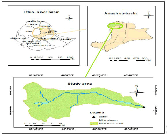
Figure 1: Location map of the study area.
The Mille watershed is located below 2400 meters above sea level; its climate is classified as a cola (hot) zone. Two distinct periods dominate it. There are dry and wet times here. The dry season begins in November and lasts until April, whereas the wet season begins in June and ends in September. May and October, the latter two months, are transitional months. While October marks the change over from the wet to the dry season, may marks the change over from the dry to the rainy season. The first rainy season, the shorter of the two, lasts from mid-March to April, while the second usually starts around June/ July.
Based on the results of the ArcGIS software's soil type of mille watershed classified as chromic luvisols, eutric chcam-bisols, eutric regosols, haplic xerosols, calcaric flubisols, orthic solonchacks, eutric cambisols, leptosols, dystric nitisols, vertic cambisols and eutric cambisols (Figure 2a). However, Eutric Regosols, Calcareous Flubisols and Haplic Xerosols make up the majority of the basin. The land cover of the study area includes water, trees, agricultural land, habitat, bare land and pastures (Figure 2b). Pasture is the dominant land use in the Milles watershed [6].
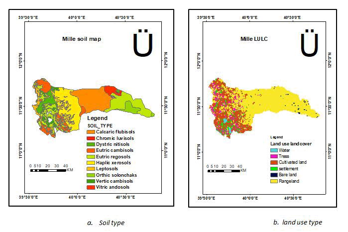
Figure 2: Soil type and land use type of Mille watershed.
Data description
The rainfall-runoff simulation input data mainly include meteorological (rainfall), hydrological (stream flow) and physiographic (land use/cover, soil type and digital elevation model) data. However, in this study, the physiographic data such as land use/ cover, land type and digital elevation model are not utilized as input for the ANN model due to its disregard for the physical characteristics of the basin. The mentioned physiographic data (land use/cover, soil type and digital elevation model) were acquired from the Ministry of Water, Irrigation and Energy to delineate the physical attributes of the study area. The primary input data for modeling the rainfall-runoff relationship using the ANN model consists of meteorological and hydrological data sourced from the Ethiopian Meteorological Agency and the Ministry of Water, Irrigation and Energy for the period spanning 2005 to 2014. The data from Mille, Wuchala, Tita, Werebabo, Haike, Bati and Meresa stations were utilized and selected based on data. Availability, including sufficient recording time and proximity to the area of interest (watershed) (Table 1) [7].
|
Station |
Data type |
Latitude |
Longitude |
|
Mille |
Precipitation, temperature (Max, Min ) |
11.41667 |
40.75 |
|
Wuchala |
Precipitation only |
11.51761 |
39.60575 |
|
Tita |
Precipitation only |
11.16582 |
39.67108 |
|
Werebabo |
Precipitation only |
11.31667 |
39.75 |
|
Haike |
Precipitation only |
11.30532 |
39.68021 |
|
Bati |
Precipitation, temperature |
11.19667 |
40.01539 |
|
Meresa |
Precipitation only |
11.66381 |
39.6605 |
Table 1: Selected meteorology station in Mille watershed.
Observed data quality testing
Hydrological modeling begins with a data quality check, which comes after data collection. This procedure reduces the number of incorrectly anticipated outcomes and gives the model precise and accurate data. Outlier testing, homogeneity testing, consistency testing and data padding were performed to assess data quality. The normal ratio approach and the regression method were used to fill the missing data for the runoff and rainfall data, respectively. Techniques such as the double mass curve and non-dimensional plots (Figure 3) were used to check the homogeneity and consistency of the data, respectively. Rainfall and runoff data were examined for possible anomalies using the Grubbs and Beck (GB) test.
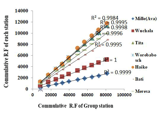
Figure 3: Double mass curve of selected metrological station.
Areal rainfall computation
Rain gauges provide measurements at specific points to show how much rain falls in a given area during a storm. In hydrological analysis, techniques such as the Thiessen polygon, isohyetal method and average station method are used to average these point measurements from different stations over a basin. In this study, the Thiessen polygon method was used. The average rainfall in the basin can be calculated using the equation.
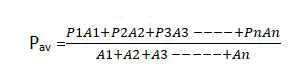
Where Pav is the average surface rainfall in millimeters, P1, P2, P3... Pn are the precipitation measurements at stations 1, 2, 3...n, and A1, A2, A3... An are the surface areas of station 1, 2, 3...n in the Thiessen polygon. Figure 4 shows the Thiessen polygon plotted for selected rainfall (Figure 5) [8].
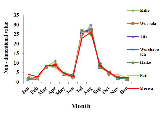
Figure 4: Non-dimensional plot for homogeneity test of the selected meteorological station.
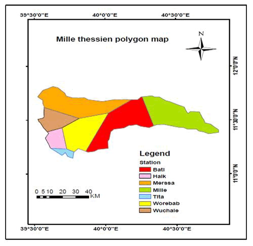
Figure 5: Created thessien polygon selected metrological station.
Artificial neural network model
The human brain cannot solve complex problems or extract information from complex structures. To address this challenge, Warren McCulloch and Walter Pitts developed a mathematical model called an Artificial Neural Network (ANN) as part of artificial intelligence. ANN is a computer system that mimics human analysis and performance, using various machine-learning algorithms to process large amounts of data. These algorithms work together in a neural network framework. The architecture of ANN is inspired by the design of biological neural networks in the human brain. The components that design the architecture of a neuron include the weights between neurons, the transfer function that controls the generation of a neuron's output, and the learning laws that determine the relative importance of the weights for a neuron's input. According to Raju et al., there are three basic classes of networks based on network architecture: Single-layer accelerated networks, multilayer networks and recurrent networks (Figure 6) [9].
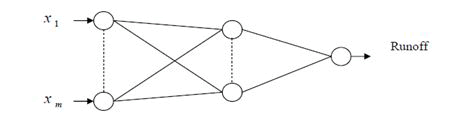
Figure 6: An architecture of multilayer perceptron.
The rainfall-runoff relationship model in this study was built using an Artificial Neural Network (ANN) with a multi-layer forward propagation network. The network was trained using a backpropagation technique. Information is processed in this network with direct propagation from the input layer to the hidden layer and from the hidden layer to the output layer. The number of neurons in the input and output layers varies depending on the specific problem, while the number of hidden layers and neurons in the hidden layer is deter-mined through a trial and error process. To predict the inputoutput relationship, each connection is assigned a synaptic weight, which represents the relative connection strength of the two nodes at both ends. The result for each node (yj) is calculated using the formula.
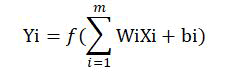
Where m is the total number of inputs to node j, bj is the threshold of the node, Wi is the weight assigned to each neuron, and Xi is the input received at node j. The activation function f, which produces the result from the weighted sum, is typically the logistic sigmoid function in most research.
In this study, the input data was transformed from the input layer to the output layer using the logistic sigmoid function, with processing taking place in a hidden layer. This sigmoid function can be found using.
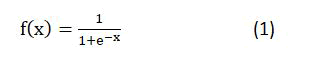
ANN rainfall-runoff modeling
In order to effectively implement Artificial Neural Networks (ANNs), it is important to assess the merits of different net-works and understand the best methods to train them. When using neural networks for rainfall and runoff modeling, several decisions need to be made. In this study, MATLAB 2019b with the Neural Net Tool Package (nntool) were utilized to train and validate the ANN model for the Mille watershed rainfall and runoff process.
The following steps were taken to develop a rainfall-runoff ANN model for the Mille watershed:
Selection input parameter: The first step in developing an ANN model is selecting the appropriate inputs. For rainfall and runoff modeling with the ANN model, we considered rainfall, runoff, and lag as the inputs. It is crucial to perform correlation analysis between these input data and the target to choose the right input for the model. Therefore, autocorrelation and cross-correlation analyses were conducted for this study using SPSS software. SPSS, a statistical program, was used for data collection and examination.
Autocorrelation examines the correlation be-tween a parameter and its antecedent value (e.g., runoff with its lag), while cross-correlations are between different parameters and their antecedent values (e.g., runoff with its lag).
Data normalization and partition: Once the set of raw data has been analyzed and deemed adequate (quality and consistency checked), further pro-cessing such as data normalization can be implemented. This involves adjusting the data to a specific range, such as [0, 1], [-1, 1], etc., to prevent computational issues and facilitate network learning. After the model is trained and tested, the results are converted back to their original units of measurement. It is given by
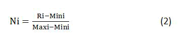
Where Ri represents the real value applied to node i; Ni represents the standardized value calculated for node i; Mini is the minimum value of all values applied to node i, and Maxi is the maximum value of all values applied to node I (Table 2).
| Data | Training period | Mean | SD | Testing period | Mean | SD | ||
| Min | Max | Min | Max | |||||
| Rainfall (mm) | 0 | 71.3 | 1.93 | 5.47 | 0 | 42.16 | 1.95 | 4.38 |
| Flow (m3/s) | 0 | 715.7 | 9.7 | 37.26 | 0.36 | 215.4 | 5.14 | 26.6 |
Table 2: Statistical properties of observed rainfall and runoff data at Mille watershed during training and testing.
Following normalization, the available data set is typically divided into two parts: The training set for network training and the validation set for model validation. Therefore, the data from the first 8 years (2005-2012) are selected for training the model, and the data from the remaining 2 years (2013 and 2014) are used to test the performance of the trained model. The training set contains input data and target (output) data, while the test set contains only input data.
Model training: After sorting the data, the neural network is created by adjusting the weights that connect its neurons. To begin training, the ANN architecture and training parameters are first adjusted. The number of input and output nodes depends on the specific training task. According to Marcoulides, determining the number of nodes in the hidden layer can be a challenging task. The number of layers and neurons in the hidden layer are typically determined through a trial and error approach. For this study, the number of hidden nodes in the hidden layer was determined through a trial and error Approach, ranging from one to twenty hidden nodes. In this study, FFNN was used to train the ANN model for rainfall and runoff modeling, which is commonly done in most studies using the error inversion algorithm. During training, the parameter value was repeatedly adjusted within an allowed range until the simulated value closely matched the observed value. The ANN model training phase was completed when the root mean square error was minimized and the R value was maximized in the regression plot. The training process was stopped when R (all) remained unchanged. The ANN model with R approaching one and MSE approaching zero between the selected epochs was adopted for further testing (cross-validation).
Testing the network: Network testing involves running the trained model with independent data (i.e., data not used in the training process) and evaluating the results similarly to the evaluation procedure in model training. In this study, data from 2013 to 2014 were used to test the model formed for runoff modeling. Unlike model training, model testing only involves input data and not a target.
Evaluation of model performance: In the present study, the model performance was evaluated using three methods during the calibration and validation periods.
Nash and Sutcliffe Simulation Efficiency (NSE): The Nash- Sutcliffe Efficiency (NSE) factor is a measure of forecast model accuracy. It is calculated by subtracting the sum of the squared differences between the predicted and observed values from 1, and then dividing by the variance of the observed values. This factor is commonly used in hydrology and other fields to evaluate a model's performance in predicting future values.

Where: Oi is observed flow, Pi is predicted flow and Pavg is the average predicted flow.
Root Mean Square Error (RMSE): RMSE is a measure commonly used to quantify the deviation between the values predicted by a model and the actual values observed in the modeled environment. The RMSE calculation involves:

Where: QO is observed flow, QP is predicted flow and N is Total No of data
Correlation of determination (R2): The coefficient of determination is a statistical measure that determines the degree to which variation in one variable can be explained by variation in a second variable when predicting the outcome of a specific even.
General methodology
In this study, we used an empirical model (artificial neural network) to determine the relationship between rainfall and runoff in the Mille basin. The first step of the methodology involves collecting data, including spatial, hydrological and meteorological data from various institutions such as the Ministry of Water Resources, Irrigation and Energy (MOWIE) and the National Meteorological Agency (NME). Once the data has been collected, the general methodology is summarized in the Figure 7.

Where: Oi is observed flow, Pi is predicted flow, Oavg is average observed flow, Pavg is average predicted flow.
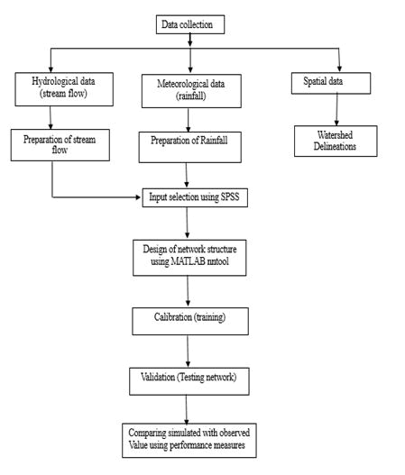
Figure 7: Flow chart showing the general methodology of the study.
Results and Discussion
SPSS correlation result
The selection of input variables is crucial in building an accurate ANN model as the model's prediction heavily relies on the chosen inputs. To identify suitable input variables for leakage, autocorrelation and cross-correlation results from SPSS were utilized. By analyzing the correlation between precipitation, runoff and their respective delays, input variables that significantly affect the model's performance were identified, while those with little impact were excluded. The input variables were selected based on their Pearson correlation values, with a value of r indicating the strength of the linear relationship between two quantitative variables. If 0
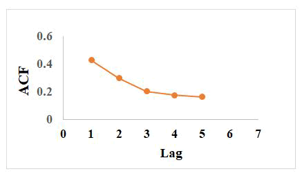
Figure 8: Auto-correlation function of runoff with its lag.
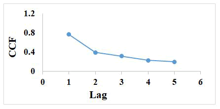
Figure 9: Cross-correlation function of runoff with rainfall and its lag.
In daily rainfall-runoff modeling, the cross-correlation between the runoff and rainfall time series as duplicated in Figure 9 showed pt and pt-1 have a Pearson correlation value of 0.768 and 0.402 with runoff respectively. So pt and pt-1 have a high and medium correlation with runoff respectively. The autocorrelation of the runoff time series, shown in Figure 8 runoff values up to lag 1 have a medium correlation. Rainfall and runoff above one day lag have no significant influence on run-off, so they are not considered input variables for the ANN model during rainfall-runoff modeling. Therefore, the main input parameters for the ANN model are actual rainfall, one-day delayed rainfall, and one-day delayed runoff (Pt, Qt-1, and Pt-1). Where Q (t)=flow at time t, Pt=precipitation at time t, Qt-1, Qt-2, Qt-3, Qt-4, and Qt-5 are the flow at t-1, t-2, t-3, and t-4, and Pt-1, Pt-2, Pt-3, Pt-4, and Pt-5 respectively. These inputs are used to model the rainfall-runoff relationship of the Mille watershed with ANN, through three combinations of input variables: M1, M2 and M3.
M1 consists of a single node in the input layer and the output layer, with the nodes representing the precipitation and runoff of the same day, respectively. In other words, Q(t)=f(Pt).
M2 consists of two nodes in the input layer, representing the precipitation of the same day and the rainfall of the previous day, with flow in the output layer. That is, Q(t)=f(Pt, Qt-1).
M3 consists of three nodes in the input layer, representing the same day's precipitation, the previous day's runoff and the previous day's precipitation, with flow in the output layer. That is Q(t)=f(Pt, Qt-1, Pt-1).
ANN model training result
To analyze the rainfall-runoff ratio of the Mille catchment, we created an artificial neural network using the multi-layer perceptron backpropagation (MLFFP) algorithm with a sigmoid transfer function. The network consists of three layers: Input, hidden and output. The number of hidden neurons was determined through trial and error, evaluating different combinations of inputs with varying numbers of neurons (ranging from 1 to 20) in the hidden layer (Table 3). The input layer incorporates daily precipitation (Pt), one-day precipitation (Pt-1), and runoff delay (Qt-1). We normalized the input-output datasets to a range of 0 to 1 to prevent saturation using the sigmoid activation function. The performance of the ANN model for the Mille basin was assessed by observing the R and MSE values during the training and validation phases, helping us choose the appropriate neurons for the hidden layers with different inputs (Table 4).
|
Performance rating |
R2 |
NSE |
|
Very good |
0.65<R2<1 |
0.65<NSE<1 |
|
Good |
0.55<R2<0.65 |
0.55<NSE<0.65 |
|
Satisfactory |
0.4<R2<0.55 |
0.4<NSE<0.55 |
|
Unsatisfactory |
R2<0.4 |
NSE<0.4 |
Table 3: General performance rating for recommended for daily time steps.
| Parameter | Value |
| Number input | 1-3 |
| Number neurons in hidden layer | 1-20 |
| Number of hidden layer | 1 |
| Transfer function | log sigmoid |
| Training algorithm | Back propagation |
| Epochs | 1000 |
| Training goal | 0 |
| Momentum factor | 0.001 |
Table 4: Parameter of ANN architecture used to create ANN rainfall-runoff model for Mille watershed.
Comparison of model results using performance indices
In Figure 5, the performance index values of three potential ANN rainfall and runoff models are illustrated during the training and testing period. According to Moriasi, Arnold, van Liew, Bingner, Harmel, the three potential ANN models are highly accurate, with a determination coefficient of more than 0.65 in the daily simulation. The objective of this study is to select the best ANN model to model the rainfall-runoff relationship of the Mille watershed. To choose the best model, it is important to compare the three models with the value of the performance index. Among the three potential ANN models, M2 has a higher performance index value and is selected as the best ANN model for modeling the rainfall-runoff relationship of the basin. In Table 5, M2 has a coefficient of determination of 0.82 during the training phase and 0.78 in the testing phase, which indicates good compatibility between the simulated flow and the observed flow. The RMSE is 12.9 m3/s during the training phase and 8.1 m3/s during the testing phase. The Nash and Cliff efficiency coefficients are 82.37% and 74.7% during training and testing, respectively. Based on performance evaluation criteria, it is concluded that M2 is the best ANN model for accurately deriving the rainfall-runoff relationship in the Mulle watershed. The statistical properties of the observed and sim-ulated flow of the M2 model during training and testing are presented in Table 6. The model shows a tendency to under-estimate during training and overestimate during testing (Table 7).
| Model | Model input parameter | Number of input parameter | Number of neurons in the hidden layer | Output layer | Model structure |
| A | Q(t)=f(Pt) | 1 | 12 | 1 | 1 12 1 |
| B | Q(t)=f(P(t), Qt-1) | 2 | 10 | 1 | 2 10 1 |
| C | Q(t)=f(Pt, P(t-1), Qt-1) | 3 | 20 | 1 | 3 20 1 |
Table 5: Input parameter and final selected ANN structure for rainfall-runoff modeling for Mille watershed.
| Model | Training (2005-2012) | NSE | Testing (2013-2014) | NSE | ||
| R2 | RMSE | R2 | RMSE | |||
| M1 | 0.74 | 18.9 | 99.9 | 0.72 | 16.4 | 87.8 |
| M2 | 0.82 | 12.9 | 82.37 | 0.78 | 8.37 | 74.7 |
| M3 | 0.81 | 16.31 | 80.84 | 0.74 | 10.3 | 74.4 |
Table 6: Performance indicator value of Mille ANN rainfall-runoff model during training and testing period.
| Statistical property | Training | Testing | ||
| Observed (m3/s) | Simulated (m3/s) | Observed (m3/s) | Simulated (m3/s) | |
| Minimum | 0 | 0.23 | 0.36 | 2.4 |
| Maximum | 715.7 | 693.8 | 215.4 | 279.14 |
| Average | 9.7 | 10.9 | 5.14 | 6.37 |
| Standard deviation | 37.26 | 33.37 | 26.6 | 17.3 |
Table 7: Summery statistical properties of Mille rainfall-runoff modeling result in training and testing.
The regression plot analysis
The model randomly divides the data into training, testing and validation sets during training. The number of neurons in the hidden layer was adjusted to train the model. The selected model is determined by examining the R value in the regression plot. The trained model's performance is dis-played in a regression plot of the model's output against the target in the nntool train data manager. Figure 10 shows a regression plot of the observed and predicted excursion during the training, testing and validation phase for the chosen M1 model. From the regression plot, it was concluded that the predicted flow developed by different input parameters performs better and closely matches the observed data sets.
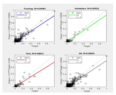
Figure 10: Dialogue box showing training performance of selected ANN model (M2).
Graphical comparison of observed and simulated runoff of (M2)
In addition to the performance indicators mentioned, a set of graphical indicators was developed to evaluate the model during training and testing. Figure 11 presents a hydrograph (time series graph) and Figure 12 shows the scatter plot of observed and simulated runoff of model M2 during training phases. Figure 11 demonstrates a good correlation between the observed and simulated runoff results during model training. Furthermore, the hydrograph indicates that the flow observed is lower than the runoff simulated during training. The observed runoff and simulated runoff results are more closely related to the 450 line in Figure 12, indicating that the results during model training are well-matched with each other. Figure 13 and Figure 14 illustrate the time series and scatter plot of the simulated and observed leakage value of an M2 model during all test phases. Figure 13 demonstrates that the flow values observed during model testing are highly consistent with those measured. The hydrograph also shows that most of the simulated runoff is greater than the runoff observed during the test. As depicted in Figure 14, the simulated and observed flow appear nearer to the line marked by an area (450) at most points, suggesting that there is a good correlation between the values of the simulation and the observed value during model testing. By using graphical indicators, the study was able to demonstrate that an ANN model can accurately predict the rainfall patterns of Mille watershed.
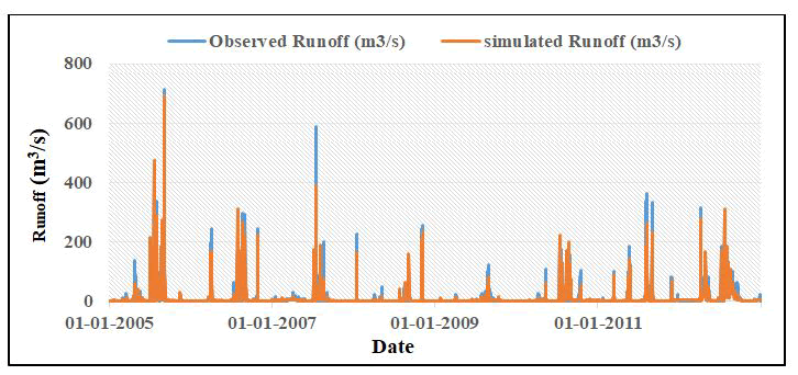
Figure 11: hydrograph comparing observed and simulated runoff of M2 model during training.
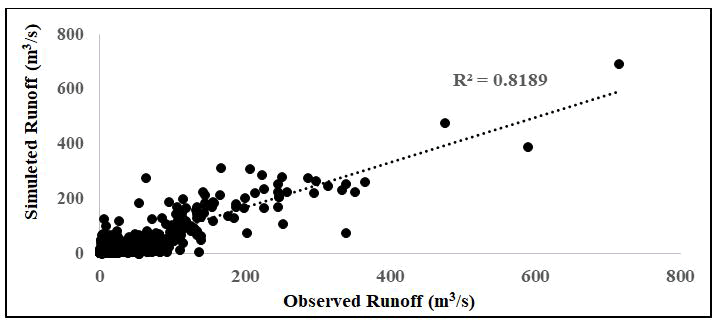
Figure 12: Scatter plots comparing simulated and observed runoff of M2 model during training.
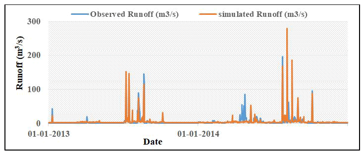
Figure 13: Hydrograph comparing observed and simulated runoff of M2 model during testing.
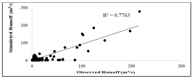
Figure 14: Scatter plots comparing simulated and observed runoff of the M2 model during testing.
Conclusion
In this study, a daily rainfall-runoff ANN model with a feedforward back propagation network is developed for the mille watershed, Awash Basin, Ethiopia. Runoff strongly correlates with present rainfall, previous one-day rainfall, and runoff in the Mille watershed. From the selected daily ANN model, the regression plot between observed and simulated runoff as well for the Mille watershed. The performance of the selected model was evaluated by statistical performance indicators such as Coefficient of determination (R2), Root Mean Square Error (RMSE), and Nash Sutcliff Efficiency (NSE). The results from the research indicate that the ANN model has a very good ability to extract the relationship between rainfall and runoff of the mile watershed. Based on the result of the testing phase, the coefficient of determination (R2) and Root Mean Square Error (RMSE) performance measures were: M1: 0.72, 816.4 (M2) 0.78, 8.37 (M3) 0.74, 10.3. From this result, M2 gives the highest performance. In addition to performance indicators the performance of the model was also assessed graphically by hydrograph and scatter plot. It is seen from the hydrograph and scatter plot graph that the observed runoff has very good agreement with simulated runoff. Due to its simple structure and high performance, the developed model (M2) which consists of one input in the input layer, 10 hidden nodes in the hidden layer and one output in the output layer is recommended for mille rainfall-runoff modeling. The result of this study provides useful information for water resource problem studies in the Mille watershed and another large river basin of Ethiopia.
Conflict of Interest
The author declares that there is no conflict of interest regarding the publication of this paper.
Data Availability
The data sets generated during and/or analyzed during the current study are available from the corresponding author upon reasonable request.
Acknowledgments
The author would like to express his gratitude Ethiopian Ministry of Water and Energy and the Ethiopian Meteorological Service Agency for providing stream flow and rain-fall data.
References
- Tokar AS, Markus M (2000) Precipitation-runoff modeling using artificial neural networks and conceptual models. J Hydrol Eng 2000: 156-161.
- Abdul Razad AZ, Sidek LM, Jung K, Basri H (2018) Reservoir inflow simulation using MIKE NAM rainfall-runoff model. J Eng Sci Technol 13: 4206-4225.
- Aoulmi Y, Marouf N, Amireche M (2021) Assessment of artificial neural network rainfall-runoff models under different meteorological inputs: Case study of Seybouse basin, Northeast Algeria. J Water Land Develop 50: 38-47.
- Chow VT, Maidment DR, Mays LW (1998) Applied hydrology. McGraw-Hill, New York, pp. 1-294.
- Moriasi DN, Arnold JG, van Liew MW, Bingner RL, Harmel RD, et al. (2007) Model evaluation guidelines for systematic quantification of accuracy in watershed simulations. Transactions of the ASABE 50: 885-900.
- Dar LA (2017) Rainfall-runoff modeling using artificial neural network technique. Int Res J Eng Technol 4: 424-427.
- Dawson CW, Wilby RL (2001) Hydrological modelling using artificial neural networks. Prog Phys Geogr 25: 80-108.
- Demirel MC, Venancio A, Kahya E (2009) Flow forecast by SWAT model and ANN in Pracana Basin, Portugal. Adv Eng Softw 40: 467-473.
- Devia GK, Ganasri BP, Dwarakish GS (2015) A review on hydrological models. Aquat Procedia 4: 1001-1007.