Spanish
  Chinese
  Russian
  German
  French
  Japanese
  Portuguese
  Hindi
Hindi Research Article, J Hydrogeol Hydrol Eng Vol: 12 Issue: 2
Numerical Modeling of a Complex and Data-Limited Wetland Catchment: Multi-objective Calibration and Validation
Bahaa-eldin EA Rahim1* and Yusoff I2
1Department of Geology, Auburn University, Alabama, USA
2Department of Geology, University of Malaya, Kuala Lumpur, Malaysia
*Corresponding Author: Bahaa-eldin EA Rahim
Department of Geology, Auburn University, Alabama, USA
E-mail: bahaa_wali@yahoo.com
Received date: 11 December, 2022, Manuscript No. JHHE-22-83071;
Editor assigned date: 14 December, 2022, PreQC No. JHHE-22-83071 (PQ);
Reviewed date: 28 December, 2022, QC No. JHHE-22-83071;
Revised date: 13 February, 2023, Manuscript No. JHHE-22-83071 (R);
Published date: 22 February, 2023, DOI: 10.4172/2325-9647.1000257
Citation: Rahim BEA, Yusoff I (2023) Numerical Modeling of a Complex and Data-Limited Wetland Catchment: Multi-objective Calibration and Validation. J Hydrogeol Hydrol Eng 12:2.
Abstract
By their nature, wetlands represent an ecosystem base for many concurrent heterogeneous interactions where the mission of numerical modeling requires a wide range of consistent and reliable datasets from a variety of different sources, spatially and temporally. However, such a mission usually collides with the existence of tremendous missing in time series dataset (s), the thing that undermines the key processes of model performance evaluation, namely calibration and validation. In this context, mike she was used to construct an integrated surface subsurface flow model for the Paya Indah wetlands in Malaysia where huge gaps exist in the historical datasets of water level and flow rate. To calibrate and validate the model to a satisfactory level, a tri-criteria simulation approach was applied to overcome the occasional missing values in these datasets. This goal was accomplished by calibrating the surface water level and channel flow while simultaneously matching the steady state subsurface portion of the system wherever water table depth data allowed. Quantitatively, the integrated model scored the highest values of R (0.765-0.927) and CE (0.748-0.828) during the validation. However, large RMSE values were calculated for the flow rate during calibration at SWL2 (outlet; 0.766) and during validation at Langat river (0.780). This bias was attributed to low or occasional absence of variation in the historical time series datasets necessary for the simulation process. Furthermore, visual assessment revealed that the hydrographic dynamics characteristics (especially for surface water) were represented better by the model during the validation period than the calibration period.
Keywords: Mike she modeling; Lake-aquiferinteraction; Wetland conservation; Peat land; Evapotranspiration
Introduction
Depending on the availability, variability and spatial representativeness of the input parameters and on the weight attributed to each hydrologic component of the water cycle, hydrological models as useful tools for water resource management are meant to demonstrate satisfactorily accurate simulation of some or all of the hydrological processes occurring within a watershed [1]. In fact, wetland ecosystems worldwide are generally not understood adequately owing to their complex ecohydrological nature, whereby periodic fluctuations of surface water and groundwater head increase the complexity of the hydrological system of such watersheds. The functionality of using multiple criteria instead of single calibration target for hydrological models, which was established using different modeling codes and a variety of input parameters, depends on the quality and representativeness of the calibration datasets. In most cases, such models failed to represent precisely the dynamic water level in shallow aquifers owing to unsatisfactory base flow simulation and oversimplified parameterization of the unsaturated flow which eventually led to replacement of conceptual groundwater modules with external coupled surface water groundwater models [2].
The multi-criteria calibration approach was found to have satisfactory performance for catchment hydrological models. Such models, which include mike she and swat, require a multi-objective calibration process to compensate scarcity in both temporal and spatial datasets and to overcome model limitations that might produce biased output [3]. Even though adjustments between several criteria are crucial to balance conflicting objectives, it remains difficult to identify an optimal dataset; consequently, the multi-criteria simulation approach is required to consider different calibration targets concurrently [4].
The full-integration criterion requires a wide range of input parameters, high heterogenetic levels of spatial distribution and a linear time varying system. This, in turn, might dramatically increase the chance of occurrence of some major calibration issues such as over parameterization, equifinality and model structure uncertainty, the very thing that raises the threshold of acceptability for users [5]. Many attempts have been made to overcome the limitations of mike she model performance, including addressing calibration issues through the inclusion of an uncertainty analysis method that enabled the model to solve and satisfactorily interpret the entire range of ecohydrological processes.
Nevertheless, the major challenges linked to mike she model calibration, especially for medium to large scale catchments, might derive from the complex nature of the study site in question and limitations of the input data. In such situations, for optimal model performance, it is crucial to curb unreliable judgments by maintaining similarities between the model and reality during the calibration processes using different sets of targeted parameters.
By their nature, wetlands are a complex ecohydrological system where the mission of numerical modeling requires a wide range of consistent and reliable time series datasets from a variety of different sources. However, such a mission usually collides with the existence of huge gaps in historical datasets, which in turns undermine the key processes of model performance evaluation, i.e. calibration and validation. In practice, routine collection of hydro meteorological data is rare in many wetlands or watersheds because of the problem of vandalism. Consequently, measurements in such regions are almost invariably limited to a single site or, at most, to a small number of locations [6-8]. Accordingly, the spatial variability of hydrological conditions might not be maintained, which is the thing that most affects the satisfactory application of distributed hydrological models to the simulation of spatially variable processes. Furthermore, in wetland hydrological models, data limitations mostly necessitate.
• The application of a simple approach, e.g., interpolation for rainfall and observed time series water level fluctuations.
• The adoption of certain uniform values, e.g., for potential evapotranspiration.
However, these options can result in overall bias in model productivity, especially when huge discontinuity is encountered in the observational dataset of one or many of the calibration targets [9]. The approach of adopting multiple calibration targets allows better use of the available input dataset, regardless of its consistency, for simulation of hydrological processes by maintaining a satisfactory level of conformity between the different targets through the statistical measures embedded in the model. Thus, the auto calibration process becomes most effective when there is variability of the calibration targets [10]. This study, therefore, aimed to overcome limitations in observational data continuity by increasing the number of calibration targets, as well as the number of simulation points for each target to be validated later using accurate field datasets.
Materials and Methods
Study area
The region of the Paya Indah Wetlands (PIW) is located in the Kuala Langat district in the state of Selangor, Malaysia (as shown in Figure 1). It covers an area of ~242 km2 and it encompasses myriad ecosystems, e.g., old tin mining ponds and peat swamp forest. The study area forms part of the Langat river basin, which consists of metamorphosed sandstone, shale, mudstone and schist. In the low flatlands, thick quaternary deposits that lie on the bedrock are distributed along the coastal fringe.

Figure 1: Description of the study area.
Input datasets
Digitized topography dataset Jurukur Permata Malaysia, 2003 was used to generate a 20 m contour map (Figure 2a). Soil types in Figure 2b together with the spatial hydraulic properties sets for each type. Rainfall time series sets from Oct 1999-September 2004 (calibration) and August 2007-August 2008 (validation) [11]. The rainfall input for the model was distributed spatially according to a weighted method in which the total rainfall was calculated from the measured rainfall and area weighted factors in Figure 2c and 2d. The data were then converted into the mike she time series format.

Figure 2: a) Distribution of spot level dataset and topographic model of PIW catchment; b) Soil sampling and in situ measurements spots and modeled soil map for PIW catchment; c) Estimated rainfall fields for the catchment using thissen polygon method; d) Land use map of the Paya Indah wetland catchment; e) Flooded areas within of the Paya Indah.
Potential Evapotranspiration (ETp) was estimated as a function of ET0 by means of a crop coefficient, i.e., ETp=ET0 × kc,
Where;
kc =Crop coefficient.
The MIKE SHE code estimates the actual Evapotranspiration (ETa) based on the model of Kristensen and Jensen.
The MIKE SHE model required the Leaf Area Index (LAI) and the Root mass Distribution (RD) for each land use type. The vegetation specific parameters for the PIW were retrieved from the land use map of Kuala Langat for the years 1998 and 2006. For the PIW catchment, the total number of land used types identified was 10. The distribution of vegetation parameters were based on identification of the dominant characteristic vegetation and land use types within the basin [12]. The main impact on land use has been logging activities, especially in the area to the North of main lake where the forest has been removed and the land left barren. Such activity has been the primary cause of the decay and subsidence of the peat land blanket in this area [13].
Hydrological process
The mike she model describes hydrological processes mostly based on the laws of conservation of mass, momentum and energy. The 1D and 2D diffusive wave Saint Venant equations are used to describe channel and overland flow, respectively. The methods of Kristensen and Jensen Refsgaard, are used for evapotranspiration, the 1D equation of Richards is used for the unsaturated zone flow and a 3D Boussinesq equation is used for the saturated zone flow (Table 1). These partial differential equations are solved using finite difference methods, while other methods (namely, interception/evapotranspiration and snowmelt) in the model are based on empirical equations obtained from independent experimental research [14].
Table 1: Properties of vegetation within the Paya Indah wetland catchment.
Model domain and discretization
Numerically, the area was discretized into a mesh of 200 m × 200 m that comprising 6500 cells. The total number of computational cells in the groundwater model was approximately 19,500. The hydraulic model is overlain by both the unsaturated zone model and the overland flow model.
The model uses Cassini coordinates of Selangor state in Malaysia in metric units. Despite the relatively coarse discretization of 200 m × 200 m, it appears suitable for calculating the overall water balance and the impact of large scale developments. Such as in the town of Cyberjaya adjacent to the Northeast corner of the catchment However, the model could easily be refined or zoomed in models created.
Overland flow and detention storage
Overland sheet flow occurs when the water depth on the ground surface exceeds 2 mm. Other than surface topographic elevation, detention storage and the roughness coefficient (manning’s number; N), the required input data for the surface water model (mike 11 model) consists of branch networks, cross sections, control structure geometry and operation schedules. The model area is dominated by reasonably flat peat swamp with little topographic relief. Therefore, overland flow was considered of little importance in the peat swamp where the undulating ground surface restricts surface flow [15]. However, for the other types of soils, the overland flow direction and velocity were determined based on the ground surface slope and the roughness coefficient. The dimensionless values of manning’s number assigned for the flow rate in PIW catchment ranged between ‘5’ for he peat swamp and ‘10’ for channels.
Flooded areas
To describe flow attenuation and surface water storage, information on floodplain dynamics was crucial for simulation of river floodplain interaction. Accordingly, with the exception of the narrow tongue at the Northeastern corner of the PIW catchment, the ground surface of the Kuala Langat swamp forest was generally considered flat with a number of flooded areas (lakes), floodplains and depressions [16]. The Paya Indah lake system was assigned as a flooded area with a code given for each lake, whereas the depression and floodplain data were derived from the topographical model by comparing riverbank elevations with surrounding surface elevations.
Hydrogeological parameters
A 3D conceptual geological model consisting of three layers was developed (Figure 3) using ArcGIS 10.8. The hydraulic properties of aquifers and the vadose zone and their spatial distribution beneath the PIW were determined from geological profiles based on a comprehensive hydrogeological investigation conducted in this area. In fact, over the previous few decades of extensive tin mining activities within the study area, the original geological formation, especially around the lake areas, has been covered completely by secondary mining deposits. Hydrogeologically, PIW model comprises of three geological layers which are, from top to bottom, peat (≈ 8 meter), silty clayey sand (≈ 20 meter), and silty sandy gravel (≈ 30 meter). Numerically, hydraulic properties for each layer including hydraulic conductivity, transmissivity, and storage and leakage coefficients datasets were used to develop the geological model.

Figure 3: Conceptual model for the PIW.
The low hydraulic conductivity of layer 2 (aquitard) indicates that the PIW lake system is not in direct hydraulic contact with the aquifer, which in turn proves that the lakes do not recharge the aquifer. This conclusion is supported by the fact that these lakes have been filled with mining material (clays/silts) that is characterized by very low hydraulic conductivity (9.95 × 10⁻⁷ m/s to 1.2 × 10⁻⁸ m/s). Furthermore, the large hydraulic gradients observed in the Paya Indah lake system (different lake water levels) would not be possible under natural conditions if the lakes were settled in highly permeable soils, especially during periods of little or no inflow to Paya Indah. The horizontal conductivity of the aquifer ranges between 1 × 10⁻³ m2/s and 3.3 × 10⁻⁵ m2/s. The vertical conductivity estimated to be (0.1) × (value of horizontal conductivity measured for each layer) [17]. The storage coefficient ranges from 0.001/m to 4.5 × 10⁻⁵/m. Withdrawal of groundwater was specified at four production wells with depths of 55 m-60 m. For base flow estimation, the value of 0.001 was assigned for the specific yield of the shallow aquifer of layer 1 (unconfined aquifer). For layer 3 (deep aquifer), a storage coefficient value of 4.5 × 10⁻⁵/m was assigned.
Calculation
Water movement in the unsaturated zone
As a basic assumption, water flow in the unsaturated zone can occur as a Darcy flow within the soil matrix, as a gravity flow in distinct macropores (macropore flow), or as a matrix flow regime that can be described by Richards’s equation;
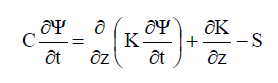
Where;
C=Soil water capacity (mm-1),
ψ=Pressure head (mm),
K=Saturated hydraulic conductivity (mm s-1),
z=Gravitational head (mm) and S=Root extraction sink term (s-1).
Therefore, water movement in unsaturated soil is governed by an equation that can be derived by combining Darcy’s law with the principle of mass conservation. The pressure head form of the equation for a 1D vertical flow is;
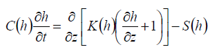
Where;
C(h)=Differential water capacity ( ∂θ/∂h) (L−1),
θ=Volumetric water content (L3/L3),
h=Soil water pressure head (matrix) (L),
t=Time (T),
z=Vertical coordinate (L),
K=Isotropic hydraulic conductivity (L/T) and
S=Sink term that represents root water extraction (L3/L3/T).
In this study, the simplest approach was applied, which involved establishing a mass balance for the root zone and calculating the average moisture content for the entire root zone. If a sufficient amount of water is available within the root zone or in the capillary fringe, the simulated actual evapotranspiration is equal to the potential rate. In a water shortage situation, the potential rate reduces to a function of the available soil moisture within the root zone. Although the model has the benefits of being simple to use and fast to run, it is still based on physical soil properties [18]. The lower boundary condition for the unsaturated zone in the model simulates the groundwater potential head. Hence, the depth of the unsaturated zone changes dynamically depending on climatic and hydrologic conditions.
Assessment of calibration procedure
Given the complexity and limited data situation of the PIW catchment reflected in the calibration procedure of the distributed parameters, the calibration process aimed to obtain a set of model parameters that could provide satisfactory agreement between model results and field observations. In this context, three main groups of input datasets were selected to control the accuracy of the calibration process. These inputs included.
• The saturated hydraulic conductivity, i.e. the specific yield of the aquifer of the groundwater model and the model for aquifer channel water exchange.
• The infiltration and evapotranspiration rates that were used in the 2 layers water balance of the unsaturated zone model to ensure correct simulation of the water yield volume.
• Manning’s roughness coefficient for overland grid cells and channel grid cells. Depending on the availability of the input time series datasets required for a successful calibration process, the model was calibrated against the surface water level, groundwater head and channel flow rate for the period July 1, 1999 to October 31, 2004.
Assessment of validation procedure
The validation process covered the period August 1, 2007 to August 1, 2008. The surface water level and groundwater head were validated at only eight and two locations, respectively. However, for channel flow simulation, SWL1 was replaced by Langat river owing.
• Vandalism at SWL1.
• The availability and consistency of Langat river flow data.
To maximize model performance accuracy, a no flow policy (water retention and release) was scheduled for the control gate at the lotus outlet (SWL2) during the entire validation period. In fact, this particular flow policy was intended to improve the scheduling and communication of special events on the lotus outlet (SWL2) and to maintain the primary goal of flood control and public safety.
Assessment of model performance
In this study, both qualitative (based on visual graphical technique) and quantitative (based on statistical measures) methods of assessment were combined but with greater emphasis placed on the statistical measures. The statistical measures for each point during the calibration an validation periods were evaluated in Tables 2 and 3, respectively. Furthermore, the predictive accuracy was tested using Pearson’s distribution index (r2). The MIKE SHE simulations were considered optimal if the MAE, R, RMSE and Nash-Sutcliffe Coefficient of Efficiency (CE) were close to the values of 0, 1, 0 and 1, respectively. Obviously, the PIW model scored the highest values of R (0.765-0.927) and CE (0.748-0.828) during validation. However, large RMSE values were calculated for the flow rate during calibration at SWL2 (outlet; 0.766) and Langat river during validation (0.780). This bias was attributed to low or occasional absence of variation in the historical time series datasets necessary for the simulation process. In contrast, the calibration period was characterized by some missing values in the observational data, which were therefore excluded from the statistical assessment accordingly. Actually, in terms of statistical evaluation and visual flow dynamic presentation, the best performance was achieved during the validation period, and for the surface water level and channel flow simulations in particular, rather than for the groundwater table [19]. Further mathematical explanations of these statistics can be found in the literature.
Results and Discussion
The combined use of surface water and groundwater requires a resource assessment that includes both surface and subsurface domains. In the current study, three crucial calibration targets were assigned for the simulation of the hydrological processes of the PIW catchment scale model to overcome occasional missing values in the historical datasets of surface water level, groundwater head and channel flow rate. The process was then evaluated qualitatively through visual judgment and quantitatively using a performance evaluation set embedded in the model designed to measure the level of agreement between model simulated values and observed data of the calibration targets [20].
The model was calibrated and validated against the water level at 12 and 8 locations, respectively in Figure 4. Concurrently, the flow rate was included as an additional calibration target in the simulation process at three further locations to strengthen the predictive accuracy of the model. Satisfactory performance in Table 2 was obtained in nine calibration locations at which agreement between observed and simulated water levels was well matched (correlation (R) ≥ 0.75) during the entire calibration period. The observable overestimation and underestimation trends, which occurred only during short time intervals, were attributed to the normal uncertainty associated with modeling that could possibly be due to scaling problems. However, some sharp overestimated fluctuations in water level were simulated, causing considerable mismatch (0.45 ≥ R ≥ 0.65) between observed and simulated values during the following periods (Figure 5).
• November-October 1999 (Figures 4f, 4h and 4j),
• November-March 2003 and
• August-September 2004 (Figure 4l).
It appears that an appropriate water level for the PIW lake system during special events (e.g., storms and droughts) could be maintained only if the control gate at the lotus outlet (SWL2) was opened and closed as required by the water release and reduced flow policy. Owing to the unavailability of such information regarding actual past control strategies (e.g., the setting of gate opening and maximum rate of exchange) and exact operational schedules, the model could not represent such events accurately. This is illustrated in the calibrated water level hydrographs of the Lotus-Outlet (SWL2) Figure 4l and the closest lakes, i.e., Chalet, Typha and Lotus (Figure 4f, 4h and 4j). These results reveal that drought conditions have caused the water level to drop by 20 cm-60 cm.
bConsistency of overall flow of PIW model predictions beyond its development conditions;
cRMSE units are (m) for Surface water and groundwater levels; (m3/s) for channel flow rate;
dTypha lake is considered an extension for Lotus lake;
N/A: Not Applicable;
*Significant slope values (P ≤ 0.05);
**Very significant slope values (P ≤ 0.01).
Table 2: Evaluation criteria for the calibrated model.

Figure 4: Hydrographs for simulation of surface water level during the calibration period.
The observed and simulated surface water level hydrographs during the validation period are illustrated in Figure 5. The results clearly reveal that the model response was much better during the validation period than during the calibration period in that the dynamics of the water level fluctuations are represented well. Furthermore, most of the simulated flow fluctuations match their observed counterparts well, especially for the upper and middle lakes, namely Visitor, Main, Tin, Crocodile and Hippo lakes in Figure 5a-5e and Table 3. However, at the lower lakes (namely, Chalet, Typha and Lotus), it appears that the model missed capturing two anomalous peaks that occurred during two periods.
• January 4-11, 2008.
• March 22-25, 2008 (Figure 5f-5h).
These anomalies are justified by the occurrence of an event comprising four successive storms during the first period followed by another event comprising two storms during the second period, which accounted for 8.2% and 3.2%, respectively, of the total rainfall during the entire validation period. In fact, maintaining a no-flow policy at control gate (Lotus-Outlet) during the entire validation period contributed effectively to the satisfactory representation of the dynamic characteristics of the surface water flow in comparison with the calibration period. Thus, the overall slight underestimation, especially for the lower lakes, was mainly related to the accumulation of water in Lotus lake after the storm events, which tended to exceed the discharge intake capacity of the broad crested weir type of control gate.

Figure 5: Hydrographs for simulation of surface water level during the validation period.
Results of channel flow simulation during both periods of calibration and validation are presented in Tables 3 and 4 respectively as well as in Figure 6. There is a satisfactory agreement between the modeled flow and the observed hydrograph of the Inlet during the calibration period in Figure 6a, supported by a reasonably strong relationship based on the skewness index (r2) of 0.78, and by the very significant (P ≤ 0.01) prediction variables in Table 3. These results demonstrate the reasonably close relationship between observed and simulated discharge that shows the best fitting modeled result of the PIW, which in turn demonstrate that the modeled results have higher conformity than the mean of the observed data.

Figure 6: Simulation of PIW channel flow at the inlet and outlet spots during calibration and validation periods respectively. Hydrographs a) and b) represent calibrated flow at SWL1 and SWL2 while c) and d) represent validated flow at Langat river and SWL2 respectively.
Noticeably, the modeled flow rate at the lotus-outlet didn’t match its corresponding measured one in Figure 6b, as evidenced by poor evaluation criteria (R=0.45; CE=0.42), values of distribution index (r2=021), as well as both of predictive variables of 0.35 and 0.27 for the slope and intercept respectively in Table 3. This disagreement is attributed mainly to unscheduled operations that occurred at the weir of the lotus outlet. Similar to the surface water level at this spot in Figure 4l, these operations obviously influenced the flow rate during both dry and wet periods, which accounted for the occurrence of many uncaptured limbs of the model simulated hydrograph in Figure 6b. Because of vandalism occurred for the automatic data logger at the Inlet spot, the reach of Langat River within the PIW catchment had been chosen in order to compensate the missing flow rate data during the validation period. The flow rate simulation result revealed a uniquely identical matching between measured and modeled values for the reach of Langat river stamped with some slight overestimation on some occasions (Figure 6c). Similarly, both patterns of modeled and measured flow rate at the lotus outlet Figure 6d match identically each other, clear from remarkably (P<0.01) high evaluation and prediction criteria of R=0.927; CE=0.828; r2=0.86 (Table 3).
bConsistency of overall flow of PIW model predictions beyond its development conditions;
cRMSE units are (m) for surface water and groundwater levels; (m3/s) for channel flow rate;
dTypha lake is considered an extension for Lotus lake;
N/A: Not Applicable;
*Significant slope values (P ≤ 0.05);
**Very significant slope values (P ≤ 0.01)
Table 3: Evaluation criteria for the validated model.
Noticeably, there is some logically slight misrepresentation at few simulation points observed in the lotus outlet hydrograph in Figure 6d with much attributed to standardization of the dimensionless roughness value of ‘10’ to be assigned to the whole channels of the PIW. In fact, this assigned roughness value is considered slightly high relative to tropical climate conditions of the study area, where the plant hold back rivers are the common feature associated with the watercourses. This practice was adopted in order to overcome the unsteadiness condition of the PIW model during the calibration process that popped up because of the over parameterization issue.
To further investigate the dynamic characteristics of flow at this problematic stimulation spot of lotus outlet, the behavior of flow rate relative to rainfall events illustrated in Figure 7. In response to rainfall events, the PIW model, therefore, succeeded to simulate the hydrological dynamics of the flow rate which included the overland flow as well specially from spots other than peat swamps where a very low roughness coefficient of ‘5’ was assigned in consistence with occurrence of many objects obstructing the flow dynamic including grassy vegetation and rough ground surface. Unlike small rainfall events, the model simulated the significant stormy events at its best satisfactory performance because of the insignificant contribution from OL; as there is no runoff over a thirst/unsaturated soil. Once again, the performance harmony of the validated PIW model has been interrupted by the over accumulation of water in Lotus lake after the storm events.

Figure 7: Hydrodynamic fluctuations of the modeled flow rate at lotus outlet relative to rainfall events.
The results for groundwater heads during the calibration and validation periods are shown in Figure 8, Tables 3 and 4. Five out of eight locations show good agreement between simulated and observed groundwater heads during the calibration period in terms of dynamic fluctuation. It was found that the rise and fall patterns in the piezometers at BH1, BH2 and BH3 in Figure 8a-8c, respectively are much more dynamic in the upland areas in the northern upper part of the modeled catchment in comparison with BH6, BH7 and BH8 in Figure 8f-8h, respectively that show gradual fluctuation. It seems that the groundwater head in the upper part of the catchment rose and declined abruptly in response to the periodic flow exchange between the saturated and unsaturated zones caused by seepage from the overland flow and inflows from the surrounding Kuala Langat swamp forest. These fluctuations caused the groundwater table across the modeled catchment to drop by between 0.45 m and 0.65 m during the dry season. In fact, while the measurements are point values collected at groundwater piezometers, the model simulations are representative of average groundwater headwithin an area of ~242 km2.

Figure 8: Simulation of groundwater head at PIW. Hydrographs (ah) represent calibration period. Hydrographs (i and j) represent validation period.
The groundwater head at BH3 was expected to have limited episodic influence in response to subsurface leakage from the nearby Main lake, taking into account the substantial difference of groundwater head fluctuations at BH3 and those shown for this lake in Figures 8c, 5b and 4e. Thus, no clear relation was evident between the groundwater head around BH3 and the water level of main lake that could be considered as aquifer lake interaction in this part of the catchment. However, the downstream part of the catchment that extends from Lotus lake to the reaches of the Langat river lies within the zone of influence of the megasteel pumping well field, which strongly controls the groundwater heads.
The validated model showed satisfactory spatially distributed predictions of the dynamics of groundwater head with a performance somewhat similar to that achieved during calibration for BH3 in Figure 8j, Tables 3 and 4. However, the nearly flat representation of the groundwater level in the simulation hydrograph at BH5 in Figure 8i might reflect the occurrence of some expected uncertainties in this part of the modeled catchment, mostly associated with extensive groundwater withdrawal at the Megasteel well field. This assumption is strongly supported by the fact that the simulated groundwater table tended to rise by approximately 0.2 m at BH3 in comparison with the calibration period for the same piezometer, whereas the groundwater head at BH5 dropped by approximately 0.75 m during both wet (November-January) and dry (May-July) periods (Figure 8e and 8i).
Conclusion
The approach of multi-criteria simulation was applied to overcome limitations in both continuity and availability of the observational datasets used to model a complex data limited wetland catchment. In fact, the hydrological connectivity of PIW (i.e. site specification) facilitates bridging gaps in historical datasets as the model calculates simultaneously all hydrological processes of different calibration/ validation targets. Three calibration targets including surface water level, channel flow rate and groundwater head were specified for the period July 1, 1999 to October 31, 2004. To maintain simulation of at least a single complete hydrological cycle, the calibrated coupled model was validated for the period August 1, 2007 to August 1, 2008 using an accurate field dataset. The coupled model demonstrated satisfactory simulation performance for all the hydrodynamic components of the water cycle throughout the PIW catchment. The accuracy of the model applicability to PIW was assessed by high scores of the R and CE measures. Nonetheless, large RMSE values were calculated for channel flow rate during calibration at SWL2 (outlet) and during validation at Langat river (replacement of SWL1 inlet). In fact, this bias was an inevitable outcome following vandalism and occasional absence of variation in the historical time series datasets necessary for the timely simulation process at SWL1 and SWL2, respectively.
Visual assessment and multi-criteria evaluation showed that both the calibrated and the validated models performed satisfactorily. However, the hydrographic visual assessment revealed that the dynamic characteristics, especially for surface water, were represented better by the validated model than by the calibrated model. The latter was noticeably influenced by unscheduled flow operation of the control gate at the lotus outlet. Therefore, in this study, validation is defined only as substantiation that a site specific model can perform simulations at a satisfactory level of accuracy; hence, no universal validity of the general model code is tested nor claimed. During validation, the groundwater dynamics in the area between Lotus lake and the Langat river were influenced remarkably by groundwater abstraction at the megasteel well field. The simulated channel flow for both the calibration and the validation period responded reasonably well to the input rainfall data. This showed that the water level in the lakes and channel system fluctuates in response to climatic variability. Moreover, because of the flat topography, it also has the ability to retain a significant proportion of the runoff, especially during storm events. Thus, the rate of surface water flow varies greatly from year to year and from event to event.
The flexibility of the MIKE SHE operating structure allows using of any number of components depending on the availability of input data. Discontinuity of observational time series datasets, the absence of records of actual historical and present flow control strategies, as well as the operational schedule appear to control model accuracy. However, this modeling practice demonstrates that calibrating the model against more than two targets (e.g., surface water level, streamflow, runoff, groundwater heads and groundwater discharge) could improve the predictive accuracy of model performance. Unlike conventional simplified watershed models that cannot represent all the components of the water cycle, the unique feature of the mike she hydrological components is the integration of various hydrological processes at different timescales. Thus, the nature of the integration and the ability to account for both surface and subsurface flow systems and their interactions make the mike she model well suited for wetland studies.
Acknowledgments
The authors would to thank the University of Malaya (UM) and the Department of Irrigation and Drainage of Malaysia (DID).
Conflict of Interest
The authors declare they have no conflict of interest.
References
- Adeyeri OE, Laux P, Arnault J, Lawin AE, Kunstmann H (2020) Conceptual hydrological model calibration using multi-objective optimization techniques over the transboundary Komadugu-Yobe basin, lake Chad Area, West Africa. J Hydrol Regional Studies 27:100655.
- Ahmadi M, Arabi M, AscoughII JC, Fontan DG, Engel BA (2014) Toward improved calibration of watershed models: Multisite multiobjective measures of information. Environ Model Softw 59:135-145.
- Alminagorta O, Rosenberg DE, Kettenring KM (2016) Systems modeling to improve the hydroecological performance of diked wetlands. Wat Resour Res 52:7070-7085.
- Rahim BE, Yusoff I, Abdul Rahim S, Wan Zuhairi WY, Abdul Ghani MR (2008) Heavy metal contamination of soil beneath a waste disposal site at Dengkil, Selangor, Malaysia. Soil Sediment Contam 17:449-466.
- Rahim BE, Yusoff I, Samsudin AR, Yaacob WZW, Rafek AGM (2010) Deterioration of groundwater quality in the vicinity of an active open-tipping site in West Malaysia. Hydrogeol J 18:997-1006.
- Bizhanimanzar M, Leconte R, Nuth M (2020) Catchment-scale integrated surface water groundwater hydrologic modelling using conceptual and physically based models: A model comparison study. Water 12:363.
- Beaulieu JJ, Balz DA, Birchfield MK, Harrison JA, Nietch CT, et al. (2018) Effects of an experimental water level drawdown on methane emissions from a eutrophic reservoir. Ecosystems 21:657-674.
[Crossref] [Google Scholar] [PubMed]
- Choi YS, Choi CK, Kim H, Kim KT, Kim S (2015) Multi-site calibration using a grid based event rainfall–runoff model: A case study of the upstream areas of the Nakdong river basin in Korea. Hydrol Process 29:2089-2099.
- Gutpa HV, Sorooshian S, Yapo PO (1998) Toward improved calibration of hydrologic models: Multiple and noncommensurable measures of information. Wat Resour Res 34:751-763.
- House AR, Thompson JR, Acreman MC (2016) Projecting impacts of climate change on hydrological conditions and biotic responses in a Chalk valley, Riparian wetland. J Hydrol 534:178-192.
- Im S, Kim H, Kim C (2009) Assessing the impacts of land use changes on watershed hydrology using mike she. Environ Geol 57:231-239.
- Jaber FH, Shukla S (2012) MIKE SHE: Model use, calibration, and validation. Trans ASABE 55:1479-1489.
- Ji H, Fang G, Yang J, Chen Y (2019) Multi-objective calibration of a distributed hydrological model in a highly glacierized watershed in Central Asia. Water 11:554.
- Kristensen KJ, Jensen SEA (1975) Model for estimating actual evapotranspiration from potential evapotranspiration. Nord Hydrol 6:170-188.
- Legates DR, McCabe GJ (1999) Evaluating the use of ‘‘goodness-of-fit’’ measures in hydrologic and hydroclimatic model validation. Wat Resour Res 35:233-241.
- Liu J, Liu T, Bao A, de Maeyer P, Feng X, et al. (2016) Assessment of different modelling studies on the spatial hydrological processes in an arid alpine catchment. Wat Resour Manag 30:1757-1770.
- Ma L, He C, Bian H, Sheng L (2016) MIKE SHE modeling of ecohydrological processes: Merits, applications, and challenges. Ecol Eng 96:137-149.
- Mehdi R, Latif K, Mohamed MH (2018) An integrated approach for modeling wetland water level: Application to a headwater wetland in coastal Alabama, US. Water 10:879.
- Nguyen VT, Dietrich J (2018) Modification of the SWAT model to simulate regional groundwater flow using a multicell aquifer. Hydrol Process 32:939-953.
- Parra V, Arumi JL, Munoz E (2019) Identifying a suitable model for low-flow simulation in watersheds of South-Central Chile: A study based on a sensitivity analysis. Water 11:1506.