Spanish
  Chinese
  Russian
  German
  French
  Japanese
  Portuguese
  Hindi
Hindi Research Article, J Hydrogeol Hydrol Eng Vol: 14 Issue: 1
Performance Evaluation of Satellite Rainfall Data in the Bheri River Basin, Nepal
Bikalpa Poudel*and Mukesh Kafle
Department of Civil Engineering, Institute of Engineering, Tribhuvan University, Lalitpur, Nepal
*Corresponding Author: Bikalpa Poudel
Department of Civil Engineering, Institute of Engineering, Tribhuvan University, Lalitpur, Nepal
E-mail: bikalppoudel@gmail.com
Received date: 09 April, 2024, Manuscript No. JHHE-24-145270;
Editor assigned date: 12 April, 2024, PreQC No. JHHE-24-145270 (PQ);
Reviewed date: 29 April, 2024, QC No. JHHE-24-145270;
Revised date: 06 February, 2025, Manuscript No. JHHE-24-145270 (R);
Published date: 13 February, 2025, DOI: 10.4172/2325-9647.1000364.
Citation: Poudel B, Kafle M (2025) Performance Evaluation of Satellite Rainfall Data in the Bheri River Basin, Nepal. J Hydrogeol Hydrol Eng 14:1.
Abstract
Nepal is a mountainous country with very difficult terrain so, there are not available Meteorological stations. In such conditions, Satellite Precipitation Products (SPPs) can be used for water resources studies. The Bheri River Basin is studied in this research. Hydrological model is developed for the Bheri River Basin using HEC-HMS. Calibration and Validation was done with ground rainfall data at two stations, Jamu and Samaijighat. For the calibration, the values of NSE, PBIAS and R2 were 0.73, -12 and 0.77 at Jamu and 0.80, -5.5 and 0.83 at Samaijighat. For the validation, the values of NSE, PBIAS and R2 were 0.70, 0.3 and 0.72 at Jamu and 0.80, -3.9 and 0.81 at Samaijighat. For the same model, performance of the model was evaluated by measuring NSE, PBIAS and R2 by providing bias adjusted GPCP1DD rainfall data which resulted in satisfactory model performance at Jamu and good at Samaijighat.
Keywords: SPPs, Bheri River Basin, GPCP1DD, Bias adjusted, Calibration, Validation
Introduction
Understanding the hydrological processes taking place in a river basin is aided by hydrological modeling of the basin. With the development of multiple types of hydrological models, scenario analysis and hydrological simulations of watershed dynamics have become more practical. Hydrological models such as HEC-HMS, SWAT, MIKE-SHE, HBV, etc. are available [1]. HEC-HMS stands for Hydrologic Engineering Center-Hydrologic Modeling System, developed by the US Army Corps of Engineers [2]. The entire hydrologic cycle of dendritic watershed systems is simulated by HECHMS [2].
Nepal is a Mountainous country. Nepal lies in between latitude 26° 22’ N to 30° 27’ N and longitude 80° 4’ E to 88° 12’ E. The geographical topography of Nepal is very different within small distance. So, there is high variation in rainfall pattern. The availability of data for hydrological modeling is limited by poorly spaced rainfall gauge networks and small number of observation years in remote and hilly areas [3]. Satellite based rainfall data are widely utilized because they are easily available and can address the limitations of ground rainfall gauge stations. Some of the examples of satellite based rainfall data are Integrated Multi-satellite Retrievals for GPM (IMERG), Tropical Rainfall Measuring Mission (TRMM) Multisatellite Precipitation Analysis (TMPA), Climate Hazards group InfraRed Precipitation with Stations (CHIRPS) and Precipitation Estimation from Remotely Sensed Information using Artificial Neural Networks for Climate Data Record (PERSIANN-CDR) [4].
Several studies of SPPs have been studied in different parts of Nepal for their applicability. In different elevation range of Nepal, among PERSIANN-CDR, TMPA, IMERG and CHIRPS, the performance of PERSIANN-CDR was good than other rainfall products [4]. The performance of APHRODITE and MSWEP V2.8 were better than CHIRPSV2.0 in the Arun river basin. In the Karnali river basin, the TMPA product was found to be used as an alternative rainfall product. In West Rapti river basin, among various SPPs the performance of IMERG was found best. The applicability of different precipitation products has been studied in different river basins of Nepal but it is found that Global Precipitation Climatology Project One-Degree daily precipitation product has not been studied. Studying the strength of GPCP-1DD in nearby regions, among 10 different SPPs, GPCP-1DD performed well in the Chitral River Basin, Pakistan. Among TMPA, PERSIANN-CDR and GPCP-1DD, GPCP-1DD outperformed than others in the Vietnam river. So, this research aims to fill the research gap by evaluating the performance of GPCP-1DD.
Considering agriculture and water resource, the Bheri river basin is an important basin of Nepal. Different water resource projects are in developing phase in this basin. So, the applicability of GPCP-1DD in the Bheri river basin will be studied in this research.
Materials and Methods
Study area
The Bheri River basin lies in between latitude 28° 20’ N to 29° 25’ N and longitude 81° 16’ E to 83° 41’ E. The Bheri river is one of the major tributaries of the Karnali river. Its length is about 400 km long. The area of the Bheri river basin is 13,870 sq km [5]. The three main tributaries of the Bheri river are Thuli Bheri, Sani Bheri and Uttar Ganga. The Bheri river is fed by rainfall and snow melt from mountain [5]. Figure 1 shows the study area of the Bheri river basin.

Figure 1: Study area.
Digital Elevation Model (DEM) is a prerequisite for basin modeling [6]. It represents ground surface terrain in digital format. Different properties of basin like Basin area, River length, basin slope, etc., are extracted from DEM and are applied in HEC-HMS model.
A 30 m resolution raster DEM was used for this study, developed by USGS (United States Geological Survey). The projected coordinate system of this study is WGS 1984 UTM Zone 44 N. The DEM of the Bheri river basin is shown in the Figure 2 below.

Figure 2: DEM of the Bheri river basin at Jamu.
Data
For evaluating the performance of GPCP-1DD with ground rainfall gauge stations data, daily rainfall data from the period of 1st Jan 1997 to 31st Dec 2015 has been selected (Table 1). Ground rainfall stations data are obtained from Department of Hydrology and Metrorology (DHM), Nepal and rainfall data of GPCP-1DD is downloaded from website (Figure 3) [7].
The hydrological stations used for the study are:
| S. no. | Station no. | Location | Latitude | Longitude | Elevation (m.) | Data range |
| 1 | 269.5 | Samaijighat | 28° 31' 02" N | 81° 39' 25" E | 500 | 1997-2006 |
| 2 | 270 | Jamu | 28° 45' 20" N | 81° 21' 00" E | 246 | 1997-2006 |
Table 1: Hydrological stations in Bheri river basin.

Figure 3: Hydrological stations in Bheri river basin.
The methodology for obtaining the main objective of the study is divided into three steps. First step consists of extraction of GPCP-1DD rainfall data and evaluating those data with respect to ground rainfall data based on the statistical indices. Second step consists of determining the applicability of GPCP-1DD rainfall by simulating GPCP-1DD rainfall data in the calibrated hydrological model and comparing its result with the observed discharge and finally, evaluating the energy generation of selected hydropower projects from GPCP-1DD rainfall data with respect to simulated ground rainfall data. The overall methodology for the completion of this study is given in the Figure 4.

Figure 4: Methodological framework.
Evaluation of GPCP-1DD rainfall
Extraction of GPCP-1DD rainfall: We downloaded the rainfall data of GPCP-1DD from [7]. Then, we extracted the required rainfall data for the same location of the ground rain gauge stations of the Bheri river basin.
Bias Adjustment of GPCP-1DD: Random biases are expected to exist in raw SPPs. Therefore, bias adjustment is applied to SPPs prior to evaluation. We have used Climate Data Bias Corrector (CDBC) tool to remove the existing bias in raw rainfall data. The CDBC tool uses quantile mapping technique for bias adjustment. After correcting the bias in Global Climate Model (GCM) rainfall data using this tool, the performance was good with respect to the ground rainfall data [8]. This tool can be downloaded for free on GitHub website [9].
Evaluation of raw GPCP and bias adjusted GPCP: Evaluation of GPCP-1DD rainfall has been done based on statistical indices i.e., Categorical Statistical Indices (CSI, FAR, FBI and POD) and continuous statistical indices (RMSE and PBIAS).
In terms of measures relating to performance, we have assessed how well Satellite Precipitation Products (SPPs) detect precipitation in comparison to different measurements from rain gauges. The following criteria are used to identify heavy precipitation:
- "True" when a daily rainfall of ≥ 1 mm is shown by both SPPs and rain gauge data.
- "False" when GPCP indicate rainfall in non-rainy days with respect to observed rainfall
- "Miss" when GPCP does not detect rainy days with respect to observed rainfall
- "Inclusive" when both GPCP and ground rainfall data detects daily rainfall <1 mm
With the above criteria CSI, FAR, FBI and POD are calculated as follows:
- Critical Success Index, CSI=T/(T+M+F)
- False Alarm Ratio, FAR=F/(T+F)
- Frequency Bias Index, FBI=(T+F)/(T+M)
- Probability of Detection, POD=T/(T+M)
In the above parameters, T means True, F means False and M means Miss.And the continuous statistical indices are evaluated by following measures:
Root Mean Square Error (RMSE): By comparing the variations between the GPCP rainfall and observed rainfall, RMSE gives information on the performance of GPCP [10-15]. Smaller the value of RMSE better is the performance of GPCP. It is calculated by:
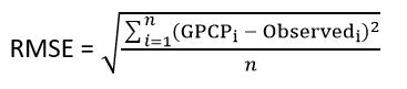
where, GPCPi and Observedi are individual rainfall data of GPCP and ground station and n is the total number of data
Percent Bias, PBIAS: PBIAS measures the mean difference between GPCP and observed rainfall data and evaluates the performance of GPCP with respect to observed rainfall [16]. It is calculated by:
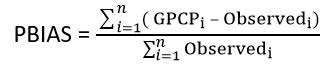
where, GPCPi and Observedi are individual rainfall data of GPCP and ground station
Assessing the performance of GPCP-1DD in hydrological model
For assessing the applicability of GPCP-1DD, we evaluated the performance of this rainfall data in HEC-HMS model. First of all, the hydrological model of the Bheri river basin is developed by confirming calibrating and validating process with the observed data [17]. Then, the model is driven with GPCP data as an input and evaluation is done on the basis of performance parameters of the simulated discharge with respect to observed discharge (Figure 5).

Figure 5: HEC-HMS model of the Bheri river basin.
Result and Discussion
Evaluation of raw GPCP and bias adjusted GPCP
The box plot of categorical statistical indices and continuous statistical indices for the evaluation of performance of raw GPCP and bias adjusted GPCP is shown the Figure 6 below:

Figure 6: Categorical statistical indices for raw and bias adjusted GPCP.
From above Figure 6, bias adjusted GPCP has better critical success index than raw GPCP while for detection of rainfall event, raw GPCP performed better than bias adjusted GPCP. Considering false alarm ratio, bias adjusted GPCP has lower value of FAR than raw GPCP which means bias adjusted GPCP has lower false detection of rainfall than raw GPCP. As FBI of raw GPCP is greater than 1, raw GPCP has overestimation of rainfall events [18].
From Figure 7, it is seen that in terms of both RMSE and PBIAS, bias adjusted GPCP showed better performance than raw GPCP.
So, from the overall evaluation of performance based on statistical indices, bias adjusted GPCP showed better performance and hence it is used for further study in hydrological model [19].

Figure 7: Continuous statistical indices for raw and bias adjusted GPCP.
Effectiveness of biased GPCP for hydrological application
The precipitation data of biased adjusted GPCP and observed data were driven in the model for determining their effectiveness for reproducing hydrological conditions. The step wise process is given below:
Calibration and validation of the model: For the calibration of the model, simulation was done from 1st January 1997 to 31st December 2002 and for the validation of the model, simulation was done from 1st January 2003 to 31st December 2006 at Jamu and Samaijighat stations respectively. The result is shown below:
From the below Figure 8, it is seen that model was calibrated at Jamu with NSE, PBIAS and R2 values as 0.73, -12 and 0.77 respectively and validated with NSE, PBIAS and R2 values of 0.7, 0.3 and 0.72 respectively [20]. Similarly, from Figure 9, for Samaijighat station, model was calibrated with NSE, PBIAS and R2 values as 0.8, -5.5 and 0.83 respectively and validated with NSE, PBIAS and R2 values of 0.8, -3.9 and 0.81 respectively. This addresses the model performance was very good at both stations.

Figure 8: Calibration and validation at Jammu.

Figure 9: Calibration and validation at Samaijighat.
From Figure 10, the scatter plot between the simulated and observed discharge at Jamu and Samaijighat stations can be seen which resulted good correlation [21].

Figure 10: Scatter plot of simulated and observed discharge at Jamu and Samaijighat.
Performance of model with biased adjusted GPCP
The daily rainfall data of bias adjusted GPCP was driven in the calibrated model for determining its performance. The performance of the model with its rainfall data as an input is shown below.
From the below Figure 11, bias adjusted GPCP driven model at Jamu showed NSE, PBIAS and R2 values of 0.47, -13.5 and 0.63 respectively. This addressed satisfactory performance of the model at Jamu with bias adjusted GPCP as an input [22].

Figure 11. Biased GPCP at Jamu.
From the above Figure 12, bias adjusted GPCP driven model at Samaijighat showed NSE, PBIAS and R2 values of 0.57, -11 and 0.72 respectively. This addressed good performance of the model at Samaijighat with bias adjusted GPCP as an input [23].

Figure 12: FDC of Biased GPCP at Jamu.
From the below Figure 13, bias adjusted GPCP driven model at Samaijighat showed NSE, PBIAS and R2 values of 0.57, -11 and 0.72 respectively. This addressed good performance of the model at Samaijighat with bias adjusted GPCP as an input [24].

Figure 13: Biased GPCP at Samaijighat.
Figures 13 and 14 show the flow duration curve of Bias adjusted GPCP and Observed data at Jamu and Samaijighat stations to see how much similar is the flow curve between them. At both stations, Bias adjusted GPCP fails to capture the peak flow [25]. The extreme flows are also overestimated by GPCP whereas, good performance in capturing medium flows and low flows.

Figure 14: FDC of biased GPCP at Samaijighat.
Bias adjusted GPCP failed to capture the peak flow [26]. It is possible that the temporal resolution (1 day) and spatial resolution (1° × 1°) of GPCP is insufficient to record short duration high intensity rainfall event that cause peak flow. From the FDC of both stations, it is seen that the extreme flows are overestimated than the observed discharge. Considering the safety, GPCP-1DD rainfall data can be used for flood forecasting, risk assessments and infrastructure designs because overestimation is always better than underestimate (Tables 2-9) [27].
| Sub Basin | Longest flow path, length (km) | Longest flow path slope (m/m) | 10-85 flow path length (km) | 10-85 flow path slope (m/m) | Area (km2) |
| 1 | 89.915 | 0.052038 | 67.436 | 0.038911 | 964.15 |
| 2 | 67.662 | 0.065428 | 50.746 | 0.044062 | 1005 |
| 3 | 66.404 | 0.059996 | 49.803 | 0.045358 | 688.65 |
| 4 | 64.991 | 0.058653 | 48.743 | 0.03623 | 1446.6 |
| 5 | 134.314 | 0.02888 | 107.485 | 0.024569 | 2801.5 |
| 6 | 60.773 | 0.058875 | 45.579 | 0.044274 | 883.46 |
| 7 | 141.77 | 0.041772 | 106.327 | 0.028318 | 1009.9 |
| 8 | 89.614 | 0.020298 | 67.21 | 0.005237 | 2679.9 |
| 9 | 90.694 | 0.020718 | 68.02 | 0.004851 | 648.17 |
| 10 | 62.333 | 0.022877 | 46.749 | 0.010824 | 1237.3 |
Table 2: Characteristics of sub basins.
| Reach | Length (km) | Slope (m/m) |
| R30 | 36.07 | 0.016634 |
| R50 | 59.718 | 0.012676 |
| R80 | 38.835 | 0.003116 |
| R230 | 72.8 | 0.00261 |
| R90 | 65.519 | 0.0029 |
Table 3: Characteristics of reach.
| Sub basin | Initial storage (%) | Maximum storage (mm) | Crop coefficient |
| 1 | 7.5 | 7.5 | 1 |
| 10 | 5 | 7.575 | 1 |
| 2 | 7.5 | 7.5 | 1 |
| 3 | 7.5 | 7.5 | 1 |
| 4 | 5 | 7.575 | 1 |
| 5 | 7.5 | 7.5 | 1 |
| 6 | 5 | 7.57 | 1 |
| 7 | 5 | 7.5751 | 1 |
| 8 | 5 | 7.5748 | 1 |
| 9 | 5 | 7.5751 | 1 |
Table 4: Simple canopy.
| Sub basin | Initial storage (%) | Maximum storage (mm) |
| 1 | 9 | 7.5751 |
| 10 | 6 | 11.306 |
| 2 | 9 | 7.575 |
| 3 | 9 | 7.5743 |
| 4 | 6 | 11.306 |
| 5 | 9 | 7.5751 |
| 6 | 6 | 11.287 |
| 7 | 6 | 16.875 |
| 8 | 6 | 7.575 |
| 9 | 6 | 7.5738 |
Table 5: Simple surface.
| Sub basin | Initial deficit (mm) | Maximum deficit (mm) | Constant loss rate (mm/hr) |
| 1 | 7.5 | 7.5 | 0.1515 |
| 10 | 7.575 | 7.575 | 0.15149 |
| 2 | 7.5 | 7.5 | 0.2261 |
| 3 | 7.5 | 7.5 | 0.15142 |
| 4 | 7.575 | 7.575 | 0.15149 |
| 5 | 7.5 | 7.5 | 0.1506 |
| 6 | 7.5699 | 7.5699 | 0.15147 |
| 7 | 7.575 | 7.575 | 0.1515 |
| 8 | 7.5748 | 7.5748 | 0.15143 |
| 9 | 7.5751 | 7.5751 | 0.15149 |
Table 6: Deficit and constant loss.
| Sub basin | Time of concentration (hr) | Storage coefficient (hr) |
| 1 | 41 | 72 |
| 10 | 31 | 59 |
| 2 | 30 | 52 |
| 3 | 31 | 58 |
| 4 | 29 | 54 |
| 5 | 32 | 60 |
| 6 | 24 | 45 |
| 7 | 29 | 53 |
| 8 | 32 | 60 |
| 9 | 34 | 52 |
Table 7: Clark unit hydrograph.
| Sub basin | Jan | Feb | Mar | Apr | May | Jun | Jul | Aug | Sep | Oct | Nov | Dec |
| 1 | 11 | 6 | 6 | 10 | 8 | 4 | 4 | 16 | 12 | 18 | 17 | 12 |
| 2 | 11 | 6 | 6 | 10 | 8 | 4 | 3 | 17 | 12 | 18 | 16 | 12 |
| 3 | 11 | 6 | 6 | 10 | 7 | 4 | 4 | 12 | 11 | 18 | 17 | 11 |
| 4 | 11 | 7 | 11 | 10 | 8 | 5 | 4 | 25 | 12 | 18 | 17 | 14 |
| 5 | 12 | 6 | 10 | 12 | 8 | 4 | 4 | 47 | 22 | 21 | 20 | 18 |
| 6 | 11 | 6 | 10 | 11 | 7 | 4 | 3 | 15 | 12 | 17 | 18 | 12 |
| 7 | 11 | 7 | 9 | 10 | 8 | 4 | 3 | 17 | 12 | 18 | 18 | 13 |
| 8 | 12 | 6 | 10 | 11 | 8 | 4 | 4 | 46 | 21 | 20 | 19 | 18 |
| 9 | 11 | 6 | 11 | 9 | 7 | 5 | 3 | 11 | 10 | 17 | 17 | 11 |
| 10 | 11 | 7 | 9 | 11 | 8 | 4 | 4 | 22 | 10 | 18 | 18 | 13 |
Table 8: Monthly base flow (m3/sec).
| Reach | Muskingum K (hr) | Muskingum X | No. of sub reaches |
| R230 | 43.006 | 0.03 | 1 |
| R30 | 39.564 | 0.139 | 1 |
| R50 | 47.656 | 0.3275 | 1 |
| R80 | 95.996 | 0.04 | 1 |
| R90 | 44.665 | 0.1 | 1 |
Table 9: Muskingum routing.
Conclusion
The applicability of GPCP1DD rainfall data is evaluated in the Bheri River Basin on the basis of performance and magnitude based indices. The major conclusions from this study are as follows;
On direct comparison with ground rainfall data, regarding multiple statistical performance indicators, quantile mapping bias adjusted GPCP-1DD resulted improvement in the performance than raw GPCP-1DD.
Bias Adjusted GPCP-1DD driven HEC-HMS model for the Bheri river basin produced satisfactory performance at Jamu with NSE, R2 and PBIAS values of 0.47, 0.63 and -13.5 and good performance at Samaijighat with NSE, R2 and PBIAS values of 0.57, 0.72 and -11. It showed good performance in capturing medium flows and low flows but it overestimated the extreme flows. Considering safety, GPCP-1DD rainfall data can be used for flood forecasting, risk assessments and infrastructure designs.
References
- Daniel EB, Camp JV, LeBoeuf EJ, Penrod JR, Dobbins JP, et al. (2011) Watershed modeling and its applications: A state-of-the-art review. Open J Hydrol 5: 26-50.
- Feldman AD (2000) Hydrologic modeling system HEC-HMS: technical reference manual. US Army Corps of Engineers, Hydrologic Engineering Center.
- Talchabhadel R, Aryal A, Kawaike K, Yamanoi K, Nakagawa H, et al. (2021) Evaluation of precipitation elasticity using precipitation data from ground and satellite-based estimates and watershed modeling in Western Nepal. J Hydrol Reg Stud 33: 100768.
- Lamichhane S, Sharma N, Devkota N (2023) Performance Assessment of Chirps, Persiann–CDR, IMERG, and TMPA Precipitation Products across Nepal. J Adv Coll Eng Manag 8: 95-108.
- Yadav SK (2002) Hydrological analysis for Bheri-Babai hydropower project–Nepal. Unpublished M. Sc. Thesis, Norwegian University of Science and Technology, Department of Hydraulic and Environmental Engineering, Norway.
- Moges DM, Virro H, Kmoch A, Cibin R, Rohith AN, et al. (2023) How does the choice of DEMs affect catchment hydrological modeling?. Sci Total Environ 892: 164627.
[Crossref] [Google Scholar] [PubMed]
- Gupta R, Bhattarai R, Mishra A (2019) Development of climate data bias corrector (CDBC) tool and its application over the agro-ecological zones of India. Water 11: 1102.
- Usman M, Ndehedehe CE, Ahmad B, Manzanas R, Adeyeri OE (2022) Modeling streamflow using multiple precipitation products in a topographically complex catchment. Model Earth Syst Env 8: 1875-1885.
- Ringard J, Seyler F, Linguet L (2017) A quantile mapping bias correction method based on hydroclimatic classification of the Guiana shield. Sensors 17: 1413.
[Crossref] [Google Scholar] [PubMed]
- Ajaaj AA, Mishra AK, Khan AA (2016) Comparison of BIAS correction techniques for GPCC rainfall data in semi-arid climate. Stoch Environ Res Risk Assess 30: 1659-1675.
- Brath A, Montanari A, Toth E (2004) Analysis of the effects of different scenarios of historical data availability on the calibration of a spatially-distributed hydrological model. J Hydrol 291: 232-253.
- Faridzad M, Yang T, Hsu K, Sorooshian S, Xiao C (2018) Rainfall frequency analysis for ungauged regions using remotely sensed precipitation information. J Hydrol 563: 123-142.
- Han WS, Burian SJ, Shepherd JM (2011) Assessment of satellite-based rainfall estimates in urban areas in different geographic and climatic regions. Nat Hazards 56: 733-747.
- Mahotra A (2023) Applicabilty of Trmm Precipitation for Hydrological Modeling Using Hec-Hms in Karnali River Basin in Nepal. J Adv Coll Eng Manag 8: 45-58.
- Vu MT, Raghavan SV, Liong SY (2012) SWAT use of gridded observations for simulating runoff–a Vietnam river basin study. Hydrol Earth Syst Sci 16: 2801-2811.
- Huffman GJ, Adler RF, Morrissey MM, Bolvin DT, Curtis S, et al. (2001) Global precipitation at one-degree daily resolution from multisatellite observations. J Hydrometeorol 2: 36-50.
- Yersaw BT, Chane MB (2024) Regional climate models and bias correction methods for rainfall-runoff modeling in Katar watershed, Ethiopia. Environ Syst Res 13: 10.
- Jiang S, Liu S, Ren L, Yong B, Zhang L, et al. (2017) Hydrologic evaluation of six high resolution satellite precipitation products in capturing extreme precipitation and streamflow over a medium-sized basin in China. Water 10: 25.
- Sikorska AE, Montanari A, Koutsoyiannis D (2015) Estimating the uncertainty of hydrological predictions through data-driven resampling techniques. J Hydrol Eng 20: A4014009.
- Cunderlik J (2003) Hydrologic model selection for the CFCAS project: assessment of water resources risk and vulnerability to changing climatic conditions. Department of Civil and Environmental Engineering, The University of Western Ontario.
- Nash JE, Sutcliffe JV (1970) River flow forecasting through conceptual models part I—A discussion of principles. J Hydrol 10: 282-290.
- Marahatta S, Devkota L, Aryal D (2021) Hydrological modeling: a better alternative to empirical methods for monthly flow estimation in ungauged basins. J Water Resour Prot 13: 254-270.
- Moriasi DN, Arnold JG, Van Liew MW, Bingner RL, Harmel RD, et al. (2007) Model evaluation guidelines for systematic quantification of accuracy in watershed simulations. Trans ASABE 50: 885-900.
- Soo EZX, Wan Jaafar WZ, Lai SH, Othman F, Elshafie A, et al. (2020) Precision of raw and bias-adjusted satellite precipitation estimations (TRMM, IMERG, CMORPH, and PERSIANN) over extreme flood events: case study in Langat river basin, Malaysia. J Water Clim Chang 11: 322-342.
- Kesarwani M, Neeti N, Chowdary VM (2023) Evaluation of different gridded precipitation products for drought monitoring: a case study of Central India. Theor Appl Climatol 151: 817-841.
- Manatsa D, Nyakudya IW, Mukwada G, Matsikwa H (2011) Maize yield forecasting for Zimbabwe farming sectors using satellite rainfall estimates. Nat Hazards 59: 447-463.
- Brunetti MT, Melillo M, Gariano SL, Ciabatta L, Brocca L, et al. (2021) Satellite rainfall products outperform ground observations for landslide prediction in India. Hydrol Earth Syst Sci 25: 3267-3279.