Spanish
  Chinese
  Russian
  German
  French
  Japanese
  Portuguese
  Hindi
Hindi Research Article, Vector Biol J Vol: 3 Issue: 1
Quantitative Structure Activity Relationships for Carboxamides and Related Compounds Active on Aedes aegypt Adult Females
Jean Pierre Doucet* and Annick Doucet-Panaye
Chemistry Department, University Paris Diderot, 15 rue Jean de Baïf, 75013, Paris, France
*Corresponding Author : Jean Pierre Doucet
Chemistry Department, University Paris Diderot, 15 Rue Jean de Baïf 75013, Paris, France
E-mail: doucet@paris7.jussieu.fr
Received: January 30, 2018 Accepted: April 03, 2018 Published: April 28, 2018
Citation: Doucet JP, Doucet-Panaye A (2018) Quantitative Structure Activity Relationships for Carboxamides and Related Compounds Active on Aedes aegypti Adult Females. Vector Biol J 3:1. doi: 10.4172/2473-4810.1000127
Abstract
Aedes aegypti mosquitoes are important vectors in the transmission of severe diseases responsible for million deaths per year. Intensive use of insecticides results in environmental damages and induced resistance in mosquitoes. Search for new molecules devoid of detrimental side effects is therefore an urgent need. In this context, we derived QSAR models for evaluating the acute toxicity of 74 carboxamides and related chemicals to females of Ae. aegypti. These models based on PaDEL, 2D topological descriptors or CODESSA, 2D/3D geometrical and quantum variables, involved multilinear regression (MLR), and various machine learning methods namely support vector machine (SVM), projection pursuit regression (PPR) and artificial neural network (ANN).
We considered first the full dataset, and then, a more homogeneous, reduced set of 50 compounds with non-conjugated carbonyl. In all cases, for data fitting and leave-one-out cross-validation, satisfactory results were attained. Good performance was also obtained for extended validation sets. Generally speaking, the modeling methods were broadly equivalent. PaDEL 2D descriptors worked better than 2D/3D CODESSA descriptors. A hybrid model combining the two descriptor sets gave improved results. Setting such QSAR models, linking activity to structural features of examined chemicals, will be of interest for prioritizing experimental tests on new candidates, and evaluate their toxicity and potential synergist effects.
Keywords: Aedes aegypti; QSAR models; Carboxamides; MLR; Machine learning methods: SVM; PPR; ANN
Introduction
Aedes aegypti mosquitoes are important vectors in the transmission and widespread of severe human pathogens (dengue, chikungunya, yellow fever and recently Zika) responsible of several million deaths per year worldwide [1,2]. Apart from repellents, avoiding bites by preventing adult mosquito to detect human odour [3], control can be carried out according to two main avenues [4,5]: larvicides (perturbing the metamorphosis process or inhibiting chitin synthesis) [6-9] in aquatic media or adulticides killing the terrestrial imagos [10-15]. However repeated and intensive use of these compounds induced an increased resistance of mosquitoes to these substances and led to environmental contamination. New insecticides with more specific action and devoid of detrimental side effects are therefore urgently needed. As a part of our concern regarding mosquito control, we proposed, in a preliminary paper [11] a QSAR (Quantitative Structure Activity Relationship) model for the toxicity of 33 piperidines to Ae. aegypti. This study is now extended to a larger population of 69 carboxamides and 5 miscellaneous chemicals identified as repellents, offering a wider structural diversity.
Several QSAR models relying on 2D, topology-based, descriptors or 2D-3D descriptors, including geometrical and quantum variables, are here developed. These models rely on multilinear regression (MLR), and varied machine learning methods (SVM, PPR, ANN). Good performances are attained in data fitting (recall) and leaveone- out cross-validation. These models also possess good predictive ability. Such approaches are efficient tools for identifying and evaluating structural features responsible for toxicity. These points may be interesting for orienting the synthesis of new toxicants, and possibly useful for regulatory purposes.
Materials and Methods
Experimental data
24h LD50 values, obtained by topical application of chemicals on the mosquito females, were retrieved from Pridgeon, for 33 piperidines [12], and 34 carboxamides [13], and completed by 7 repellents [14]. This data set of 74 compounds studied in identical conditions was the basis of the present study. Additional data on 4 isobutylamide alkaloids, derived from Piper nigrum [15], not incorporated in building up the models, were also considered as a possible extension of the treatment. Data initially expressed in μg per mosquito were converted in micromole/mosquito for the QSAR treatments. The pLD50 (log 1/LD50) ranged from 1.01 (compound #21: 1-octanoyl-3-benzyl-piperidine) to 2.69 (compound #59: hexahydro- 1-(1-oxohexyl)-1-H-azepine). Compounds are identified by a unique ID number (from 1 to 78) from the original papers, irrespective of the data selection in the investigated splitting Table 1, Figure S1.
| ID pLD50 | Name |
|---|---|
| 1 2.10 | 1-(Cyclohexylacetyl)-2-methyl-piperidine |
| 2 1.97 | (2R)-1-Decanoyl-2-methyl-piperidine |
| 3 1.51 | 1-Dodecanoyl-2-methyl-piperidine |
| 4 2.25 | (2R)-1-Heptanoyl-2-methyl-piperidine |
| 5 2.34 | 1-(3-Cyclohexylpropanoyl)-2-methyl-piperidine |
| 6 2.30 | 1-[(4-Methylcyclohexyl)carbonyl]-2-methyl-piperidine |
| 7 1.76 | (3S)-1-[(1-Methylcyclohexyl)carbonyl]-3-methyl-piperidine |
| 8 2.09 | (3S)-1-(3-Cyclohexylpropanoyl)-2-methyl-piperidine |
| 9 2.01 | (3S)-1-Heptanoyl-3-methyl-piperidine |
| 10 2.09 | (3S)-1(Cyclohexylcarbonyl)-3-methyl-piperidine |
| 11 1.71 | 1-Decanoyl-4-methyl-piperidine |
| 12 1.77 | 1-(4-Cyclohexylbutanoyl)-4-methyl-piperidine |
| 13 1.90 | 1-(Cyclohexylcarbonyl)-4-methyl-piperidine |
| 14 2.29 | 1-(3-cyclohexylpropanoyl)-4-methyl-piperidine |
| 15 1.62 | 1-Dodecanoyl-4-methyl-piperidine |
| 16 2.13 | 1-(Cyclohexylcarbonyl)-2-ethyl-piperidine |
| 17 2.43 | 1-(3-Cyclohexylpropanoyl)-2-ethyl-piperidine |
| 18 2.04 | 1-Propionyl-2-ethyl-piperidine |
| 19 2.11 | 1-(3-Cyclopentylpropanoyl)-2-ethyl-piperidine |
| 20 2.48 | 1-Nonanoyl-2-ethyl-piperidine |
| 21 1.01 | 1-Octanoyl-3-benzyl-piperidine |
| 22 1.37 | 1-Undec-10-enoyl-4-benzyl-piperidine |
| 23 1.19 | 1-(Cyclohexylacethyl)-4-benzyl-piperidine |
| 24 1.39 | 1-(3- Cyclohexylpropanoyl)-4-benzyl-piperidine |
| 25 2.28 | 2-Methyl-1-undec-10-enoyl-piperidine |
| 26 2.54 | 2-Ethyl-1-undec-10-enoyl-piperidine |
| 27 1.98 | 2-Benzyl-1-undec-10-enoyl-piperidine |
| 28 2.11 | 3-Methyl-1-undec-10-enoyl-piperidine |
| 29 2.33 | 3-Benzyl-1-undec-10-enoyl-piperidine |
| 30 1.99 | 4-Methyl-1-undec-10-enoyl-piperidine |
| 31 2.26 | 4-Ethyl-1-undec-10-enoyl-piperidine |
| 32 1.55 | Piperine: (E,E)-1-Piperoyl-piperidine |
| 33 1.85 | N,N-diethyl-3-methyl-benzamide (DEET) |
| 34 2.67 | N-butyl-N-ethyl-2-methyl-benzamide |
| 35 2.61 | N-ethyl-2-methyl-N-phenyl-benzamide |
| 36 1.84 | N-ethyl-2-methyl-N-(2-methyl-2-propenyl)-benzamide |
| 37 2.16 | N-butyl-N-ethyl-2,2-dimethyl-propanamide |
| 38 1.63 | 1-(1-Azepanyl)-2,2-dimethyl-propanone |
| 39 1.29 | N-ethyl-2,2-dimethyl-N-(2-methyl-2-propenyl)-propanamide |
| 40 2.07 | N-butyl-N-ethyl-3-phenyl-propenamide |
| 41 1.89 | N-ethyl-N,3-diphenyl-2-propenamide |
| 42 1.29 | N,N-bis((2methylpropyl)-3phenyl-2-propenamide |
| 43 2.09 | N-butyl-N-ethyl-3-methyl-butanamide |
| 44 1.99 | N,N-diisobutyl-3-methyl-butanamide |
| 45 1.77 | N-cyclohexyl-N-ethyl-3-methyl-butanamide |
| 46 2.42 | N-butyl-N,2-diethyl-butanamide |
| 47 1.66 | N,2-diethyl-N-(2-methyl-2-propenyl)-butanamide |
| 48 2.15 | N,N-diisobutyl-3-methyl-crotonamide |
| 49 2.06 | Hexahydro-1-(3-methylcrotonoyl)-1H-azepine |
| 50 1.88 | N-ethyl-3-methyl-N-(2-methyl-2-propenyl)-2-butenamide |
| 51 1.66 | N-butyl-N-ethyl-3-methyl-2-butenamide |
| 52 2.44 | 1-(1-Azepanyl)-2-methyl-1-pentanamide |
| 53 2.30 | N-butyl-N-ethyl-2-methyl-pentanamide |
| 54 1.80 | (E)-N-butyl-N-ethyl-2-methyl-pentenamide |
| 55 1.70 | (E)-1-(1-azepanyl)-2-methyl-1-pentenamide |
| 56 1.53 | (E)-2-methyl-N,N-di-2-propenyl-2-pentenamide |
| 57 1.43 | (E)-N-ethyl-2-methyl-N-(2-methyl-2-propenyl)-2-pentenamide |
| 58 2.69 | Hexahydro-1-(1-oxohexyl)-)-1-H-azepine |
| 59 2.45 | N-butyl-N-ethyl-hexanamide |
| 60 2.48 | N-cyclohexyl-N-ethyl-hexanamide |
| 61 2.35 | N-ethyl-N-phenyl-hexanamide |
| 62 2.05 | N-butyl-N-methyl-hexanamide |
| 63 1.81 | N,N-diallyl-hexanamide |
| 64 2.13 | (E)-N,N-di-(2-methypropyl)-2-hexenamide |
| 65 1.91 | (E)-N-butyl-N-ethyl-2-hexenamide |
| 66 1.73 | (E)-N-cyclohexyl-N-ethyl-2-hexenamide |
| 67 1.10 | DMP |
| 68 1.87 | Picaridin |
| 69 2.35 | AI3-35765 |
| 70 1.25 | EHD |
| 71 1.60 | IR3535 |
| 72 1.50 | PMD |
| 73 2.47 | AI-37220 |
| 74 3.12 | Pellitorine |
| 75 2.35 | Guineensine |
| 76 2.25 | Pipercide |
| 77 2.34 | Retrofractamide A |
Table 1: Experimental data.
Model design and molecular descriptors
It is noteworthy that the constraints noted in a previous data set [11] remain (i.e., limited activity range, sparse occupancy of the structural domain, complex stereo-chemical and conformational problems). In a first step, the full population (74 compounds) was considered, and extension to the four isobutylamides examined. We have then considered separately the compounds with a nonconjugated carbonyl group, constituting a “reduced” population of 50 chemicals.
It might be expected that working on a more homogeneous data set would allow for grasping more precisely structural characteristics and interaction mechanisms specific of that family, and led to increased performance in modelling (and predictive ability). Data on derivatives where the carbonyl group is conjugated with either a benzene ring or a C=C bond are too limited (24 compounds) for an in depth study. For each data set (full population of 74 compounds, or reduced set of 50), two parallel series of runs were systematically carried out: use of 2D, topology-derived, PaDEL descriptors [16] or alternatively CODESSA 2D/3D descriptors [17]. In all cases, the QSARINS package [18] with ordinary least squares multilinear regression (OLS-MLR) was selected as modeling tool and for descriptor selection. With the same set of descriptors, the MLR results were then compared with three other non-linear correlation methods [19]: support vector machine (SVM) [20], projection pursuit regression (PPR) [21] and artificial neural network (ANN: three layer perceptron) [22].
A same strategy was developed in the different approaches. It consisted first in fitting the full data set (recall) without any prediction on a test set and then in evaluating the robustness of the model [23,24]. This was carried out in cross validation. The absence of chance correlation was checked by application of the QUICK rule [25] and verification of a low value for Q2Yscr (2000 runs on randomly scrambled property values).
Cross validation was first carried out by the classical leave-one-out process (loo-cv). More in-depth investigation was then accomplished in leave-some-out process (lso-cv), examining five subsets (M0 to M4) generated from the ID number of compounds modulo 5. So subset M0 encompasses compounds #5, #10, #15 … and subset M1 compounds #1, #6, #11. Note that these splitting operations are quite random. They depend only on the rank of the compounds in the data file, with no consideration on the structural features or toxicological activity. For each of these five splitting (corresponding to a ratio train/test about 80/20%), the MLR was adjusted on the corresponding training set (which “knows nothing” about the associated validation set) and then applied for prediction on this validation set. The performance was checked on these five independent subsets M0 to M4, examining the (prediction) determination coefficient R2pred and the coefficient Q2pred corresponding to Q2-F2 of QSARINS [18,24]. Within this sets, R2pred indicates how well variations of calculated values are proportional to those of the observed ones. On another hand, Q2 specifies the ratio between the residuals observed for these calculated values and those resulting from a “null model” (mean of the observed values). It indirectly informs about the predictive ability of the model. In addition to R2 (and Q2) calculations for the correlation between observed and predicted pLD50 values, prediction accuracy could be also evaluated by the root mean squared error (RMSE), or the mean absolute error (MAE) [26].
In this approach, each compound was examined four times in training (leading in fact to very close results) and once in prediction. Gathering the predicted values in a single file allowed for comparing these predictions to the observed pLD50 via a linear regression, and so, gave a global estimate of the predictive ability of the model. As indicated farther, additional confirmation may be gained using leavemany- out cross validation (statistical cross validation).
Descriptor calculation and selection
2D topology-based descriptors were calculated from the PaDEL software [16], incorporated in the QSARINS package (v-22) [18], leading to an initial pool of about 1200 descriptors. 2D and 3D CODESSA descriptors [17], calculated on geometries optimized at the semi-empirical AM1 level (Hyperchem software), amounted about 500 descriptors (constitutional, geometrical, topological, quantum-chemical). After elimination of (quasi) constant values and pruning pairs of highly inter-correlated descriptors, it remained respectively 267 (PaDEL) and 149 (CODESSA) potentially “significant” structural variables. Descriptor selection was carried out using a Genetic Algorithm-based procedure [27,28] implemented in QSARINS, starting from examination of all the possible pairs of variables and extension of the pool via the GA (generally speaking 5000 generations, chromosomes of 200 variables) [18]. GA currently leads, for a given data set, to a population of about fifty models with very close performances, but involving various different descriptors. The “winning” OLS-MLR model was selected on the basis of the best results in loo cross validation (Q2 or RMSE), satisfying the QUICK rule. The selected structural variables were subsequently used for the different models proposed.
It’s clear that the more variables used, better the recall results. However to limit the risk of overfitting, and not uselessly complicate the model, we limited the number of variables to 10 for investigating the 74 compound set, and 7 for the 50 compound set (non-conjugated carboxamides). This corresponds to a value about 1/7 for the ratio (#parameters/#compounds), better than the 1/5 ratio generally admitted to avoid overfitting.
Methods
Multilinear Regression (Ordinary Least Squares)
With easy calculations and straightforward implementation, OLS-MLR is clearly the most widespread modeling method used in QSAR/QSPR studies. Suffices it here to say that for building up a model between a dependent (univariate) variable yi (property value) and several independent variables (structural descriptors xi) for compound i
y = X b + e,
where X represents the matrix of the independent variables xi, b and e being the column vector of the coefficients and residuals respectively. The b coefficients are determined by minimizing the residuals by OLS method
b = (XT X)-1 XT y
and the calculated response Å· is
Å· = X b
Performance in recall (fitting all data in training) is characterized by the determination coefficient R2 of the correlation obtained between observed pLD50 and the corresponding structural descriptors.
Another important information attainable in MLR is the applicability domain (AD) related to “influential” objects: those that in training have an heavy importance in the definition of the model, and in prediction, points falling outside of this AD, that must be considered with caution. In the leverage approach, the influence of each object on the regression result (its “leverage”) is given by the diagonal element h of the “Hat” matrix H
H = X(XTX)-1XT
For a study involving n training samples and p variables, objects with h larger than the threshold value h* = 3(p+1) / n are considered outside the AD. Williams’ plot (standardized residuals vs Hat diagonal values h) immediately highlights points outside the AD or outliers with residuals larger than 2.5 times the standard deviation (the common norm).
Machine learning modeling methods
Machine learning methods are increasingly used in QSAR models, due to their high flexibility [19,22,29-33]. Although they generally don’t provide any, directly usable, explicit formula for property/ activity evaluation, their easy setting, rapid training and the capacity to determine the global minimum of the response surface now make them privileged approaches in QSAR/QSPR studies, and applications to nanoparticle studies recently appeared [34-38]. Several publications presented and detailed these approaches and their implementation. We only summarize their basic characteristics. Implementation of these methods and their adjustments were carried out in the framework of the Caret package [39] from the Cran-R project.org [40].
Support Vector Machine (SVM): introduced by Vapnik [20,41] and then largely used [42-47] relies on two main ideas: the first one is to privilege robustness over an optimal recall, in view of a better predictive ability. The second one is to project (thanks to a kernel function) the initial data in a higher dimensional space where it may be hoped that a linear model might work better than in the initial data space. We used the very common linear kernel, (K(x,x’) = x*x’, x and x’ being independent variables).
The model depends on two tunable parameters: the regularization constant C, trade-off between the complexity of the model and its precision (too large values tend to overfitting) and “epsilon”, an estimation of the admissible error (roughly speaking the diameter of the “insensitive tube” around the regression line, where errors can be neglected when building up the model). Some techniques have been proposed for estimating these parameters [48,49]. Working with scaled descriptor values, these parameters were here adjusted with a grid-search type procedure (ɛ varying from 0.10 to 0.40, and C from 0.25 to 16) looking for the best loo performance.
Projection Pursuit Regression (PPR) : operates on projections of the original variables along selected directions [21,33,35,36]. The regression function, linking the property to structural variables, is approximated by a sum of smooth ridge functions of these projections. An optimization routine allows for pursuing a sequence of projections revealing the most interesting data structures in the sample set.
Artificial neural network (ANN): Three layer perceptron encompasses 3 layers of elementary units (the neurons). The input layer, fed with structural descriptors transmits weighted values to the hidden layer units. On each hidden unit these scaled inputs are summed up and transmitted to the output unit through a transfer function. Biases can be added. The sum on the output unit (possibly transformed by another transfer function) gives the calculated activity value [22]. With the “nnet” program [40], the optimization process for the weights input-> hidden layers relies on the BFGS (Broyden– Fletcher–Goldfarb–Shanno) algorithm [50]. To not multiply the number of connections (which may lead to overfitting) we restricted the hidden layer to a unique neuron in order to evaluate the interest of the ANN in its simplest form.
Results
The statistical elements for the different approaches are now presented. Comparison of the methods and their results will be analyzed subsequently.
Full data set
Selected 2D PaDEL descriptors and MLR treatment: Starting from the 2D PaDEL descriptors, 10 variables were selected by MLR from the QSARINS software: In these 10 selected variables, five correspond to components of autocorrelation vectors, two to topological atom-type E-state (based on the electron mobile count), two to topological charge indices and one to Burden’s matrix. More details can be found in Table 2 [51-54]:
| Acronym | Definition |
|---|---|
| ATSC2e | Centered Broto-Moreau autocorrelation term, lag 2, weighted by Sanderson electronegativities. It corresponds to the sum, on all pairs of atoms (i,j) separated by a given topological distance, the “lag” (here two bonds), of the products of the property value associated to each atom of the pair (here Sanderson electronegativity, “e”). |
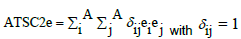 with if atoms i and j are separated by two bonds, zero otherwise and A number of atoms. with if atoms i and j are separated by two bonds, zero otherwise and A number of atoms. |
|
| MATS1c | Moran autocorrelation lag 1, weighted by charges. |
| MATS8c | Moran autocorrelation lag 8, weighted by charges. |
| GATS8c | Geary autocorrelation lag 8, weighted by charges. |
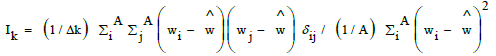
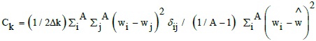
| GATS2e | Geary autocorrelation lag 2, weighted by Sanderson electonegativities. Moran and Geary autocorrelation coefficients are very similar, with centered property values (wi), but weighted by the square of the centered property value on all atoms (Moran, Ik) or all minus one (Geary, Ck). So mean and standard deviation are accounted for [51]. |
 |
|
 |
|
| A number of atoms and Δk number of atom pairs at distance k. | |
| Although looking rather similar, there are no significant inter-correlations between these variables for the data set under scrutiny. | |
| BCUTw-1l | n high lowest BCUTS eigenvalue derived from Burden’s matrix (with atomic weight on diagonal elements and, for non-diagonal ones, 0.1*traditional bond order (plus 0.1 if terminal bond) and 0.01 for non-bonded atom pairs. Other weighting schemes may imply charge polarizability or H-bond ability. |
| nsCH3 | count of atom-type E-state CH3 |
| maxHCsatu | max. atom-type H E-state H on Csp3 bonded to unsaturated C. nsCH3 and maxHCsatu belong to Roy et al. topochemical indices [52-54] based on the valence electron mobile (VEM) count. They take into account the atomic intrinsic state I of the considered atom i (depending on its electronegativity and vertex degree) and the perturbation ΔIj from the other atoms j, depending on their topological distance dij. 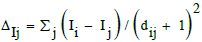 |
| GGI1 | Topological charge index of order 1. |
| JGI6 | Mean topological charge index of order 1. GGI1 and JGI6 describe the charge transfer between pairs of atoms and therefore the global charge transfer from Galvez matrix (product of the adjacency matrix by the reciprocal square distance matrix . Diagonal terms may be also replaced by Pauling electronegativity or valence vertex degree) |
Table 2: The 10 selected topology-based 2D descriptors.
• With these descriptors the following MLR model was computed:
pLD50 = 44.5505 + 0.9581 ATSC2e + 3.7912 MATS1c – 4.4874 MATS8c – 0.6636 GATS8c -2.9837 GATS2e – 3.1725 BCUTw-1l + 0.1004 nsCH3 – 0.5414 maxHCsatu – 0.2682 GGI1- 13.2384 JGI6 (1)
With fitting parameters:
R2 = 0.758, RMSE = 0.19, MAE= 0.15, s = 0.21.
And leave-one-out cross validation parameters:
Q2loo = 0.695, RMSE = 0.22, MAE = 0.17.
The small difference between R2 and Q2loo is a good indication of the robustness of the model. In parallel, the low value of Q2Yscr (for 2000 shuffled activity values; Q2Yscr = 0.138) indicates the absence of chance correlation (also confirmed with the QUICK rule).
The Relative Importance of the variables (determined from standardized coefficients in the MLR equation) decreases according to the following sequence:
MATS8c > GATS8c > GGI1 > MATS1c > GATS2e > ATSC2e > BCUTw-1l ~nsCH3 > maxHCsatu > JGI6.
Leave-Some-Out validation: Predictive ability of this model was checked on the five subsets M0-M4 defined by the ID compound modulo 5 (see above). Gathering in a single file the predicted values obtained in these five subsets (and covering therefore the whole population) a linear relationship can be established between the observed and predicted pLD50 leading to R2 = 0.708, RMSE = 0.21, MAE = 0.17.
Machine learning method treatments (2D descriptors)
For the selected machine learning methods, a same sequence was developed, using the structural variables (descriptors) previously selected from MLR: For each method: first, recall (data fitting on the global population);
then, validation (prediction on the five subsets M0-M4).
For each run, the relevant parameters were optimized: For linear SVM, parameters C (regularization) and epsilon (diameter of the error tube) were adjusted; in PPR, it was the number of projections (in fact best results were here obtained with one projection); and for ANN a unique architecture (with one hidden unit, and null decay rate in optimization) was confirmed in all trials. The main statistical results are gathered in Table 3 (including MLR for an easier comparison). Figure 1 displays a plot of calculated pLD50 values (linear SVM) vs. observed ones.
| Method Recall | Prediction | Loo C.V. | ||||||||
|---|---|---|---|---|---|---|---|---|---|---|
| R2 | RMSE | MAE | R2pr | RMSE | MAE | Q2pr | Q2 | RMSE | MAE | |
| PaDEL descriptors | ||||||||||
| MLR | 0.758 | 0.19 | 0.15 | 0.708 | 0.21 | 0.17 | 0.707 | 0.695 | 0.22 | 0.17 |
| SVM (0.10) | 0.755 | 0.2 | 0.15 | 0.707 | 0.21 | 0.17 | 0.703 | 0.703 | 0.21 | 0.17 |
| PPR | 0.799 | 0.18 | 0.14 | 0.658 | 0.24 | 0.18 | 0.642 | 0.661 | 0.23 | 0.18 |
| ANN | 0.759 | 0.19 | 0.15 | 0.694 | 0.22 | 0.17 | 0.694 | 0.667 | 0.23 | 0.18 |
| CODESSA descriptors | ||||||||||
| MLR | 0.733 | 0.2 | 0.16 | 0.606 | 0.25 | 0.2 | 0.6 | 0.644 | 0.23 | 0.19 |
| SVM (0.10) | 0.73 | 0.2 | 0.16 | 0.623 | 0.25 | 0.2 | 0.612 | 0.675 | 0.22 | 0.18 |
| PPR | 0.821 | 0.17 | 0.12 | 0.549 | 0.27 | 0.21 | 0.522 | 0.674 | 0.22 | 0.18 |
| ANN | 0.732 | 0.2 | 0.16 | 0.584 | 0.26 | 0.21 | 0.579 | 0.635 | 0.24 | 0.19 |
Table 3: Statistical parameters for the linear and non-linear approaches used. Full population: 74 compounds. For recall, prediction and loo cross-validation, determination coefficient R2, Q2, root mean squared error (RMSE) and mean absolute error (MAE) are specified. For SVM the epsilon value, indicated between brackets in the first column (Method), corresponds to both recall and loo. Prediction results refer to the correlation between experimental values and gathering the predicted ones in the five subsets Mo-M4 (with specific parameter optimization).

Figure 1: Plot of experimental and calculated (Linear SVM, 2D descriptors) pLD50 for the full population (74 compounds), in recall and prediction (predicted values are shifted up 1.5 units for the sake of clarity).
2D/3D CODESSA models
In a similar approach, 10 structural variables (over a pool of 149 2D/3D CODESSA descriptors) were selected from QSARINS. They include topological indices, geometrical parameters and quantum values, identified in Table 4.
| Acronym | Definition |
|---|---|
| C047 | Kier-Hall index order 2 2ÃÂŒ = (NSA + α-1) (NSA + α-2)2 (2P + α) 2 With NSA number of non-hydrogen atom in the molecule, 2P number of paths of length 2 in the molecular graph. α = (ri /Ci)-1 with ri and Ci radii of atom i and sp3 carbon. |
| C077 | Balaban index J = (q / µ+1) ∑ (SiSj)-0.5 with µ = cyclomatic number of the molecular graph, µ = q – n + 1 with q number of edges and n number of atoms in the molecular graph. Si distance sums calculated over rows or columns of the topological distance matrix of the molecule. Summation is over all edges ij. |
| C080 | Inertia moment C. |
| C083 | YZ shadow area. |
| C145 | HA dependant HDSA-1 (Zefirov). Hydrogen bonding donor ability of the molecule. HDSA1 = ∑DSD where D = H-donor H atom, SD solvent accessible surface area of H –bonding |
| C170 | HOMO energy. |
| C198 | Min 1-e reactivity index C atom, Fukui index RA = ∑i€A ∑j€A ciHOMO cjLUMO where c are the MO coefficients. |
| C200 | Average 1-e reactivity index for C atom. |
| C324 | FNSA-3 fractional atomic charge weighted partial negative charge surface area PNSA (PNSA-3/TMSA, Quantum) where PNSA-3 is the atomic charge weighted partial negatively charged surface area. |
| C377 | Min e-e repulsion for C-H bond 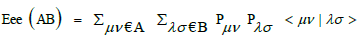 with Pμν , Pλσ density matrix elements and <μν|λσ> electron repulsion integral. with Pμν , Pλσ density matrix elements and <μν|λσ> electron repulsion integral. |
Table 4: Selected 2D/3D CODESSA descriptors.
• These 10 variables led to the following MLR model:
pLD50 = - 75.6432 - 0.223 C047 - 0.3364 C077 – 27.616 C080 + 0.0303 C83 - 0.0121 C145+ 0.591 C170 + 41.3063 C198 - 456.2506 C200 + 0.6695 C324 + 0.4939 C377 (2)
with, in recall (fitting data) R2 = 0.733, RMSE = 0.20, MAE = 0.16 s = 0.22, and
in loo cross-validation: Q2loo = 0.644, RMSE = 0.23, MAE = 0.19.
From the standardized coefficients, the sequence of decreasing importance of the terms in equation (2) is: C077 > C198 > C047 > C083 > C377 > C170 > C080 > C145 > C200 > C324.
In the William’s plot, compounds #62 and #68 are only slightly out of the applicability domain, but these two molecules remain well calculated.
• Validation: From the predicted values obtained in the five subsets, a linear relationship can be established between the observed and predicted pLD50 with
R2pred = 0.606, RMSE = 0.25, MAE = 0.20, Q2pred = 0.600.
• The same variable set was introduced in a linear SVM, PPR and ANN. Statistical results are collected in Table 3 where results for MLR were repeated for the sake of comparison.
Random Statistical Validation (Leave-Many-Out process)
To avoid a possible bias (induced by the ordering of the compounds in the data set) on the splitting into five subsets (M0 to M4), we carried out a large number of runs on random partitions test/train (about 20%/80%). MLR was chosen for correlating pLD50 with calculated values, since its performances are comparable (but not really largely superior) to the other approaches, and the method is relatively the most rapid with an easy implementation. The data set, ordered by activity, was subdivided into two parts with a frontier set at pLD50 = 1.94, leading to a subset of 34 less active compounds, and another one of 40 more active derivatives (the frontier was chosen corresponding to a light gap in the reactivity scale). In each subset, 8 compounds were randomly assigned to the test set, the others to the training set, leading to a 16/58 partition. This corresponds to a statistical validation since involving a large number of trials, with on each draw, an adjustment on the training set quite independent of the corresponding test set. Retaining only draws with R2 recall > 0.7, we found that, typically, mean values for R2pred and Q2 were about 0.690 and 0.643, with a mean MAE of 0.18 in prediction (Figure 2).

Figure 2: External statistical validation: Histograms from 2000 MLR random draws with PaDEL descriptors (full population).
With CODESSA descriptors, similar results were obtained. For example, 1000 PPR draws led to R2train = 0.783, R2pred = 0.705, Q2pred = 0.651 (not shown). These good results, simultaneously obtained in training and validation, confirm that the selected descriptors and the used approaches possess a satisfactory modeling ability.
Tentative extension to isobutylamides
Insecticidal toxicity to Ae. aegypti (pLD50 values) have been reported by Park [15] for 4 isobutylamide alkaloids derived from Piper nigrum. Prediction of the pLD50 values for these chemicals with the just proposed different models led to divergent results, depending on the selected set of structural variables. Simply looking at the chemical structures, it is worthy to note that, in isobutylamide derivatives, the nitrogen atom bears a hydrogen atom whereas, in the other investigated carboxamides, N is linked to two carbon atoms.
In MLR, with 2D descriptors, systematic large residuals (from 1.03 to 1.43) are observed, toxicity being under evaluated. A possible way to include these compounds in the model would be to introduce for isobutylamide derivatives, a supplementary indicator of about 1.2 units, which would reduce the residuals to acceptable values (< 0.30). Obviously, this correction should be verified over a larger set of chemicals (Figure 3). Conversely, using CODESSA descriptors, MLR predictions look quite acceptable for 3 of the compounds (with residuals 0.1-0.3). Only pellitorine, compound #75, predicted with a low activity (0.54) deviates of about 2.6 units! Important information on these discrepancies could be derived from examination of the applicability domain for the two MLR models. With PaDEL descriptors we checked that for the four compounds the “leverage” value (h) is largely higher than the threshold h* value (see above(§ MLR), which may explain the observed residuals. Conversely with CODESSA variables it appears that the three compounds (#76, 77, 78) are inside the applicability domain whereas compound #75 is largely outside (h = 0.86 for h* = 0.45). However, these observations must be examined with some caution. It is important to note that the average weight of Ae. aegypti female adults used by Park [15] was 1.955 mg while the weight of the female used by Pridgeon and co-workers [12-14] was 2.85 mg. Park also stressed that pellitorine could have a more rapid penetration rate in the invertebrate increasing its toxicity.

Figure 3: Piper negrum isobutylamides. pLD50 values predicted by MLR, with 2D (left) and 2D/3D (right) descriptors, using the models established on the full population. Black triangles correspond to the four isobutyl amides.
Reduced population (50 compounds)
Selection of compounds where the carbonyl group is not conjugated, with either a phenyl group or a C=C double bond, defines a more homogeneous ensemble of 50 chemicals: The same approaches as those just used for the full population were carried out: Determination of a reduced set of relevant descriptors from MLR analysis in the framework of QSARINS, and subsequent application of these variables in linear SVM, PPR and ANN. 2D PaDEL descriptors and on another hand, 2D/3D CODESSA descriptors were separately considered. Owing to the limited extent of the data set, the number of variables was limited to 7 to maintain a reasonable ratio #parameters/#compounds. These structural variables are listed in Table 5.
| Acronym | Definition |
|---|---|
| PaDEL 2D descriptors | |
| ATSC6c | Centered Broto-Moreau autocorrelation, lag 6, weighted by charge. |
| AATSC3m | Average centered Broto-Moreau autocorrelation, lag 3, weighted by mass. |
| AATSC0i | Average Broto-Moreau autocorrelation, lag 0, weighted by the first atomic ionization potential. |
| GATS6c | Geary autocorrelation, lag 6, weighted by charge. |
| GATS2e | Geary autocorrelation lag 2, weighted by Sanderson electronegativities. |
| mindsCH | min atom-type E-state = CH -. |
| maxssCH2 | max atom-type E-state - CH2 -.(Details about the signification of these acronyms, and derivation of their values have been previously specified, in Table 2, on similar descriptors). |
| CODESSA 2D/3D descriptors | |
| C145 | HA dependant HDSA-1 (Zefirov) Hydrogen bonding donor ability of the molecule. |
| C165 | final heat of formation. |
| C198 | mean 1e reactivity index for a C atom. |
| C287 | max bond order of a O atom. Bond order PAB = ∑i ∑μ€A ∑ν€B ni ciμ cjν. ni occupation number of the ith MO. |
| C295 | min valency of a C atom. |
| C320 | max e-e repulsion for a C atom. |
| C370 | max Coulombic interaction for a C-N bond. |
Table 5: PaDEL and CODESSA selected descriptors for the reduced 50 compounds dataset.
• With these 7 PaDEL variables, a good MLR is obtained for pLD50:
pLD50 = 18.533 + 2.6836 ATSC6c + 0.1096 AATSC3m – 6.3326 AATSC0i + 0.7536 GATS6c-11.6456 GATS2e + 0.3792 mindsCH – 0.928 maxssCH2 (3)
with the following statistical parameters:
R2recall = 0.863, RMSE = 0.14, MAE = 0.11, s = 0.15.
Beside the good performance in recall, robustness of the model is established by the high value of Q2 (close to R2 value) in loo cross validation, and also in leave-many-out cv (20% data left out, 2000 draws). The absence of chance correlation is also ascertained by the low value of Q2scrY (0.23) obtained on 2000 randomly shuffled runs and verified with QUICK rule.
Q2loo = 0.807, RMSEloo = 0.17, MAEloo = 0.14, Q2lmo = 0.786, R2Yscr = 0.15.
• The relative importance of the different variables decreases according to the following sequence:
GATS2e > mindsCH > GATs6c > AATSC0i ~ AATSC3m > maxssCH2 > AATSC6c
William’s plot indicates that points 62 and 40 are slightly out of the AD (but well calculated in recall).
• Similarly to the full-set treatment, validation was carried out on five subsets training/prediction. In each case, the MLR coefficients were recalculated on the corresponding training set, and the model applied to the associated set.
R2pred = 0.832, RMSE = 0.16, MAE = 0.12, Q2 = 0.830.
• With the selected CODESSA descriptors, a good MLR was also obtained
pLD50 = - 538.6369 – 0.0399 C145 + 0.0061 C165 + 34.6035 C198 + 39.1031 C287 + 114.2452 C295 + 0.213 C320 + 3.1215 C370 (4)
With R2recall = 0.795, RMSE = 0.17, MAE = 0.14, s = 0.19
Q2loo = 0.725, RMSE = 0.20, MAE= 0.17
Q2lmo = 0.680, R2Yscr = 0.15.
And in validation:
R2 = 0.741, RMSE = 0.19, MAE = 0.16, Q2 = 0.740
• The relative importance of the variables is as follows: C295 ~ C145 ~ C287 > C198 >> C370 ~ C165 > C320.
• Corresponding results obtained in linear SVM, PPR and ANN are collected in Table 6 where results for MLR were repeated for easier comparison. An example of these correlations is given in Figure 4 It may be noted that defining specific descriptors for this reduced, more homogeneous, dataset, led to more accurate results. So, for example with MLR and PaDEL descriptors, we obtained (Table 6) in recall R2 = 0.863, MAE = 0.11 and in prediction R2 = 0.832, MAE = 0.12 in place of 0.746, 0.15 (recall) and 0.699, 0.15 (prediction) respectively when evaluating the compounds of the reduced set with the general equation (1) defined on the whole set. Conversely, trying to apply to the full set the descriptors defined on the reduced set led to significantly inferior results. For the considered 24 compounds, residuals (absolute values) are systematically superior to 0.5 (for pLD50) and generally in the range 1-2.8 units. This is consistent with the fact that working on the reduced homogeneous population allowed to select specific descriptors non able to correctly describe the situation for the more diversified compounds (including conjugated chemicals).
| Method | Recall | Prediction | Loo-cv | ||||||||
|---|---|---|---|---|---|---|---|---|---|---|---|
| R2 | RMSE | MAE | R2pr | RMSE | MAE | Q2pr | Q2 | RMSE | MAE | ||
| PaDEL descriptions | |||||||||||
| MLR | 0.863 | 0.14 | 0.11 | 0.832 | 0.16 | 0.12 | 0.83 | 0.807 | 0.17 | 0.14 | |
| SVM (0.25) | 0.862 | 0.14 | 0.11 | 0.83 | 0.16 | 0.13 | 0.83 | 0.827 | 0.16 | 0.13 | |
| PPR | 0.884 | 0.13 | 0.1 | 0.802 | 0.17 | 0.13 | 0.799 | 0.782 | 0.18 | 0.15 | |
| ANN | 0.867 | 0.14 | 0.11 | 0.834 | 0.15 | 0.12 | 0.834 | 0.808 | 0.17 | 0.14 | |
| CODESSA descriptions | |||||||||||
| MLR | 0.795 | 0.17 | 0.14 | 0.741 | 0.19 | 0.16 | 0.74 | 0.725 | 0.2 | 0.17 | |
| SVM (0.30) | 0.79 | 0.17 | 0.15 | 0.745 | 0.19 | 0.16 | 0.744 | 0.752 | 0.19 | 0.16 | |
| PPR | 0.834 | 0.15 | 0.12 | 0.718 | 0.2 | 0.17 | 0.714 | 0.683 | 0.21 | 0.18 | |
| ANN | 0.801 | 0.17 | 0.14 | 0.749 | 0.19 | 0.16 | 0.749 | 0.729 | 0.2 | 0.17 | |
Table 6: Statistical results for the correlations established for the reduced population (50 Compounds).

Figure 4: Plot of experimental and calculated values (PPR with 2D descriptors) pLD50 for the Reduced set (50 compounds) in recall and prediction (predicted values are shifted up 2 units).
Conjugated carbonyl compounds
For this data set, encompassing 19 compounds, in an activity range 1.22-2.67, the same approaches were carried out. Due to the limited number of samples, this must be only considered as an exploratory treatment, restricted to MLR in recall and loo (building a test set would correspond to a sizeable loss of information). Three descriptors are however necessary for a satisfactory recall of activities. They are collected in Table 7.
| Acronym | Definition |
|---|---|
| PaDEL descriptors | |
| ATS2s | Broto-Moreau autocorrelation-lag 2, weighted by I-state. |
| ATSC5p | Centered Broto-Moreau autocorrelation-lag 5, weighted by polarizability. |
| GGI10 | Topological charge index, order10. |
| CODESSA descriptors | |
| C200 | Average 1-e reactivity index for a C atom. |
| C280 | Max Pi-Pi bond order. |
| C296 | Max valency of a Carbon atom. |
Table 7: Selected descriptors for the 19 conjugated structures.
Statistical parameters for correlations obtained in recall and loo (Table 8), are quite acceptable at least with PaDEL descriptors that, as previously observed, outperform CODESSA results. For example R2 = 0.791 with PaDEL vs. 0.697 for CODESSA variables. The difference is more important in loo cv: Q2 = 0.709 vs. 0.488 (definitively too low). This origins from some important residuals higher in CODESSA than in PaDEL: for example, compound #58 residual = 0.48 vs. -0.13, and mainly #34 0.63 vs. 0.17.
| Method Recall | Prediction | Loo-cv | |||||
|---|---|---|---|---|---|---|---|
| R2 | RMSE | MAE | Q2 | RMSE | MAE | ||
| PaDEL | 0.791 | ||||||
| MLRCODESSA | 0.16 | 0.13 | NA | 0.709 | 0.19 | 0.16 | |
| MLR | 0.697 | 0.19 | 0.16 | NA | 0.488 | 0.26 | 0.2 |
Table 8: Statistical parameters for the 19 “conjugated carbonyl” compounds.
Discussion
Generally speaking, within a given population (74 or 50 compounds) for a same set of descriptors (2D PaDEL or 2D/3D CODESSA) the performances of the four modeling methods (MLR, Linear SVM, PPR and ANN) are very comparable with highly consistent, neighboring and rather good results. Detailed results on individual patterns are collected in Table S1-Supplementary Materials. A more synthetic vision may be gained by examination of correlations existing for calculated values in prediction between methods within a same descriptor set or between sets for a given method (Table 9). Offdiagonal blocks reveal high determination coefficient observed on the corresponding predicted values obtained by the various methods with a, same set of descriptors.Upper triangle corresponds to CODESSA variables; the lower to PaDEL descriptors. Conversely, for a same method, correlation between pLD50 calculated from 2D and 2D/3D variables (diagonal cells) are of lower quality especially for the full set. This is in agreement with our previous remarks [29,47] that, for a given problem, the nature of the descriptors is more important than the choice of the modeling method. Conversely the remark on Park’s isobuylamides stresses the importance of the “applicability domain” and the fact that using different descriptor sets may be useful to get complementary information in particular situations.
| 74 compounds | 50 compounds | |||||||
|---|---|---|---|---|---|---|---|---|
| MLR | SVM | PPR | ANN | MLR | SVM | PPR | ANN | |
| MLR | 0.586 | 0.985 | 0.908 | 0.993 | 0.783 | 0.98 | 0.953 | 0.993 |
| SVM | 0.973 | 0.608 | 0.896 | 0.976 | 0.993 | 0.788 | 0.98 | 0.953 |
| PPR | 0.921 | 0.944 | 0.474 | 0.901 | 0.965 | 0.956 | 0.772 | 0.94 |
| ANN | 0.971 | 0.993 | 0.942 | 0.56 | 0.994 | 0.985 | 0.979 | 0.807 |
Table 9: Determination coefficients for inter-correlations between predicted values by different approaches (sum of the prediction over the five subsets-see text-).
Method Equivalence
Starting first from 2D PaDEL descriptors, in the reduced data set, the global statistical indices R2recall (0.86 – 0.88), Q2loo (0.78 – 0.83), Q2pred in validation (0.80 -0.83) largely outperform the usually admitted thresholds of acceptable values. With the full data set, results are a little more scattered, with slightly lower statistical criteria (although still satisfactory). (R2recall: 0.76 – 0.80, Q2loo: 0.66 – 0.70, Q2pred: 0.64 -0.71). For 2D/3D CODESSA descriptors R2recall values are close to the preceding ones whereas Q2loo and Q2pred values are less satisfactory.
This is illustrated in Figure 5 where are represented the main global statistical indices for the various methods applied for the two populations using 2D descriptors. It highlights that PPR led to slightly better results in recall and inferior in Q2pred., this behavior being more important in the full set. The same observation holds with enhanced importance with CODESSA descriptors.

Figure 5: 3D display of the main statistical parameters (R2recall, Q2pred, Q2loo) for the four correlation models (MLR, SVM, PPR, ANN) with 2D descriptors in the full and reduced populations.
Descriptors and structural information
Considering the two modes of structural description (PaDEL vs. CODESSA), generally speaking, the topological 2D descriptors give better performance, especially in prediction. A comparison of PaDEL and CODESSA selected descriptors is rather difficult since structural information is differently encoded in the two approaches. Topological-type descriptors largely rely on discrete elements of the molecular graph (atom, or bond types, pairs of atoms separated by a given distance). Quantum CODESSA variables (possibly localized on a bond or an atom) are derived from a wave function determined on the whole molecule. It may be noted that the six more important terms in equation (1) reflect the influence of charges and electronegativity for pairs of atoms distant by 8, 2 or 1 bonds. Atom types and organization of the molecular graph (depicted by Burden’s matrix) correspond to the least important terms. On another hand, with CODESSA descriptors, equation (2), organization of the molecular graph is approached via top-ranked Kier & Hall and Balaban indices. Electronic aspects intervene by the Fukui indices involving HOMO and LUMO localization. Shape is taken into account with shadow area and inertia moment.
Looking only at the two series of 10 selected descriptors it appears that, inside a given set, there are no strong correlations between them, except between C047 and C077 or C080 with R2 = 0.55. Comparing the two sets, C080 is correlated to GATS8c (R2 = 0.65), and C077 to nsCH3 (0.69). Slightly better correlations are observed if two descriptors are simultaneously considered: for example comparing C047 to the pair GATS8c, GATS2e, R2 reaches 0.61 in place of 0.46 for the “correlation” C047, GATS8c. Comparable results are obtained for C077 vs.nsCH3, GATS2e; or MATS1C vs. C047, C083.
On another hand, looking at the range of activity variations associated to the various descriptors, it appears that some terms bring contributions significantly varying over the whole population, whereas, for others, the contribution is nearly constant except a limited number of compounds; for example ATSC2E, BCUT or maxHCsatu (Figure S2-supplementary material). However, omitting these descriptors would lower the quality of the correlations, as evidenced by examination of various statistical criteria.
Efficiency and individual residuals
Beyond a simple comparison of global criteria, a more detailed analysis of performances may be approached looking at histograms of residuals (obs-calc) computed for individual compounds. The subsequent discussion will be mainly focused on MLR (which results are illustrated in Figure 6) method giving the best performances with easy implementation.

Figure 6: Histograms of residuals (MLR correlations) for the full and reduced test sets with 2D and 2D/3D descriptors. Series 1 to 6 correspond to ranges (0-0.10), (0.11-0.20) to (> 0.50). P74 and C74 stand for 74 compounds with PaDEL and CODESSA descriptors respectively; idem for P50, C50.
In such analysis, two important thresholds may be considered: 0.3 that corresponds to a ratio of 2 as to the amount (in μMol) of the lethal dose, and (here) to about 20% of the total activity range, and 0.5 (ratio of 3 for lethal dose, and 30% of total activity range). Table 10 summarizes the number and ratio of well-modeled chemicals (residuals < 0.3). In all cases, results are high, particularly with the reduced set, where they often reach or exceed 90%.
| Method | Recall | Prediction | Loo-cv | ||||
|---|---|---|---|---|---|---|---|
| FULL SET | |||||||
| PaDEL | MLR | 61 | 0.82 | 57 | 0.77 | 54 | 0.73 |
| SVM | 61 | 0.82 | 57 | 0.77 | 53 | 0.72 | |
| PPR | 59 | 0.8 | 55 | 0.74 | 58 | 0.78 | |
| ANN | 66 | 0.89 | 61 | 0.82 | 61 | 0.82 | |
| CODESSA | MLR | 55 | 0.74 | 54 | 0.73 | 52 | 0.7 |
| SVM | 55 | 0.74 | 50 | 0.68 | 51 | 0.69 | |
| PPR | 64 | 0.86 | 53 | 0.72 | 48 | 0.65 | |
| ANN | 54 | 0.73 | 58 | 0.78 | 50 | 0.68 | |
| HYBRID | MLR | 59 | 0.8 | 61 | 0.82 | 61 | 0.82 |
| SVM | 60 | 0.81 | 62 | 0.84 | 55 | 0.74 | |
| PPR | 65 | 0.88 | 61 | 0.82 | 62 | 0.84 | |
| ANN | 62 | 0.84 | 54 | 0.73 | 56 | 0.76 | |
| REDUCED SET | |||||||
| PaDEL | MLR | 49 | 0.98 | 46 | 0.92 | 49 | 0.98 |
| SVM | 48 | 0.96 | 47 | 0.94 | 48 | 0.96 | |
| PPR | 49 | 0.98 | 45 | 0.9 | 44 | 0.88 | |
| ANN | 49 | 0.98 | 47 | 0.94 | 47 | 0.94 | |
| CODESSA | MLR | 46 | 0.92 | 44 | 0.88 | 43 | 0.86 |
| SVM | 45 | 0.9 | 44 | 0.88 | 44 | 0.88 | |
| PPR | 45 | 0.9 | 44 | 0.88 | 44 | 0.88 | |
| ANN | 46 | 0.92 | 45 | 0.9 | 45 | 0.9 | |
| HYBRID | 48 | 0.96 | 47 | 0.94 | 48 | 0.96 | |
| SVM | 48 | 0.96 | 48 | 0.96 | 48 | 0.96 | |
| PPR | 50 | 1 | 47 | 0.94 | 48 | 0.96 | |
| ANN | 48 | 0.96 | 48 | 0.96 | 48 | 0.96 | |
Table 10: Number and ratio of compounds with a residual ≤ 0.30. (absolute value).
In most cases, these residuals are of comparable importance for the two descriptor sets, although generally slightly higher with CODESSA variables, both for positive or negative residual values. However for some compounds the error is definitely larger for CODESSA values (#42, 59, 62). Generally the two sets of descriptors led to deviations of the same sign (under or over - estimation) except in some cases (for example compounds #34, 46, 50) (Figure 7).

Figure 7: Residuals for MLR-predicted pLD50 with 2D PaDEL or 2D/3D CODESSA descriptors. Location of the patterns in the various quadrants (A,B), (C,D), (E,F), (G,H) indicates the sign of the residuals observed with either PaDEL or CODESSA descriptors. For example, patterns in quadrant (C,D) have a PaDEL residual, positive and a CODESSA one negative. Location of the patterns by respect to the indicated bisectors specifies if the PaDEL error is superior (or not) to the CODESSA one. For patterns in quadrant (C,D) and (G,H) the residuals are of opposite signs; hence a more efficient hybrid model.
Hybrid model
Although generally in close agreement, the two approaches (2D or 2D/3D) gave non identical results. It may be hoped, therefore, than taking the mean of the two calculated values would offer an evaluation closer to the experimental observation. The benefit would be greater in the rare cases were the deviations are of opposite signs (Figure 7) This does not correspond to a brute increase in the descriptor number (with foreseeable overfitting) but rather to a very simple type of cooperative model. Global statistical results for the three studied sub-populations are presented in Table 11.
| Method | Recall | Prediction | Loo-cv | |||||||
|---|---|---|---|---|---|---|---|---|---|---|
| R2 | RMSE | MAE | R2pr | RMSE | MAE | Q2pr | RMSE | Q2 | MAE | |
| 74 compounds | ||||||||||
| MLR | 0.805 | 0.18 | 0.14 | 0.743 | 0.2 | 0.16 | 0.741 | 0.746 | 0.2 | 0.16 |
| SVM | 0.803 | 0.18 | 0.14 | 0.746 | 0.2 | 0.16 | 0.743 | 0.763 | 0.19 | 0.15 |
| PPR | 0.872 | 0.14 | 0.11 | 0.714 | 0.21 | 0.16 | 0.713 | 0.768 | 0.19 | 0.15 |
| ANN | 0.805 | 0.18 | 0.14 | 0.729 | 0.21 | 0.17 | 0.724 | 0.664 | 0.23 | 0.18 |
| 50 compounds | ||||||||||
| MLR | 0.866 | 0.14 | 0.11 | 0.835 0.15 | 0.13 | 0.832 | 0.818 | 0.16 | 0.13 | |
| SVM | 0.864 | 0.14 | 0.11 | 0.835 | 0.15 | 0.13 | 0.808 | 0.835 | 0.16 | 0.13 |
| PPR | 0.89 | 0.13 | 0.1 | 0.81 | 0.17 | 0.13 | 0.808 | 0.796 | 0.17 | 0.14 |
| ANN | 0.867 | 0.14 | 0.11 | 0.836 | 0.16 | 0.12 | 0.834 | 0.813 | 0.16 | 0.13 |
| 19 compounds | ||||||||||
| MLR | 0.894 | 0.13 | 0.11 | NA | NA | NA | NA | 0.814 | 0.16 | 0.16 |
Table 11: Statistical results obtained with the Hybrid Model. See Table 3 caption.
As indicated in Table 11, a definite improvement in prediction (the important point for practical applications) is observed. For example, with the MLR method, as regards the full set, Q2pred = 0.743, whereas for the reduced set it is equal to 0.835, and Q2 loo for the 19 conjugated carbonyls equals 0.814.
Conclusion
Diverse approaches were developed for QSAR modeling of toxic activity to Aedes aegypti for a population of 69 carboxamides and 5 related compounds. Two sets of 10 structural descriptors (topology-based 2D PaDEL or 2D/3D CODESSA variables) relying on MLR, linear SVM, PPR and ANN, gave similar and satisfactory results for R2recall, Q2loo and R2pred, Q2pred in a in-depth validation gathering the results obtained on five subsets covering the entire population. Validity of the models was also confirmed from the statistical parameters obtained from a large number of random draws. With the availability of several evaluations for a same compound, clearly, consistent values do not guarantee a right evaluation of activity, but divergent values cast some doubt on the efficiency of the approach for this compound.
Reduction of the dataset to a population of 50 carboxamides, with a non-conjugated carbonyl, gave similar results, but of better quality (higher R2 or Q2). This is not surprising due to the more homogeneous structural space. An intriguing point, however, is that the full dataset (74 compounds) includes structures devoid of the carbonyl group or bearing also others functions. Curiously, these compounds are well modeled. In line with these observations, it may be suggested that highly homogeneous population may be modeled with specific descriptors associated to definite interactions or mechanisms. Conversely, a more diverse population would require more general descriptors possibly applicable also to other chemicals.
For these specific populations, PaDEL and CODESSA descriptors led to highly inter-correlated values for pLD50, but with better results for the PaDEL variables (except scarce examples). This prompted us to define a hybrid model where, for each approach, the activity was calculated as the mean of the values obtained with the respective PaDEL and CODESSA variables, leading to a definite improvement for calculated values.
Our models will be of interest to find new adulticides, with a moderate toxicity, to be used as synergists on pyrethroid resistant strain of Aedes aegypti.
Conflicts of interest
The authors declare no conflict of interest.
Author contributions
The authors equally contributed to this work.
This work ascarried out in the framework of project (DeltaSyn,#2101587412) from the French Ministry of Ecology, Sustainable Development and Energy
References
- Reisch MS (2016) How to contain the Zika virus. C&EN 94: 29-30
- Gubler DJ (1998) Dengue and dengue hemorrhagic fever. Clin Microbiol Rev 11: 480-496.
- Katritzky AR, Wang Z, Slavov S, Tsikolia M, Dobchev D, et al. (2008) Synthesis and bioassay of improved mosquito repellents predicted from chemical structure. Proceed Nat Acad Sci USA 105: 7359-7364.
- Devillers J, Lagadic L, Yamada O, Darriet F, Delorme R, et al. (2013) A Use of multicriteria analysis for selecting candidate insecticides for vector control In Juvenile Hormones and Juvenoids Modeling Biological Effects and Environmental Fate. CRC Press, Boca Raton, Florida, USA.
- Devillers J, Lagneau C, Lattes A, Garrigues JC, Clémenté MM, et al. (2014) In silico models for predicting vector control chemicals targeting Aedes aegypti. SAR QSAR Environ Res 25: 803-835.
- Devillers J, Doucet-Panaye A, Doucet JP (2015) Structure-activity relationship (SAR) modelling of mosquito larvicides. SAR QSAR Environ Res 26: 263-278.
- Devillers J, Doucet-Panaye A, Doucet JP (2017) SAR and QSAR modeling of structurally diverse juvenoids active on mosquito larvae In Computational Design of Chemicals for the Control of Mosquitoes and their Diseases. Devillers J ed CRC Press Boca Raton FL, USA.
- Devillers J, Doucet-Panaye A, Doucet JP, Matondo LA, et al. (2017) A SAR predictions of benzoylphenylurea chitin synthesis inhibitors active on larvae of Aedes aegypti In Computational Design of Chemicals for the Control of Mosquitoes and their Diseases. CRC Press Boca Raton FL, USA.
- Devillers J, Doucet JP, Doucet-Panaye A, Decourtye A, Aupinel P (2012) Linear and nonlinear QSAR modelling of juvenile hormone esterase inhibitors. SAR QSAR Environ Res 23: 357-369.
- Devillers J, Doucet-Panaye A, Doucet JP, Lagneau C, Estaran S, et al. (2017) Predicting the toxicity of piperidines against female adults of Aedes aegypti In Computational Design of Chemicals for the Control of Mosquitoes and their Diseases. CRC Press, Boca Raton, FL, USA
- Doucet JP, Papa E, Doucet-Panaye A, Devillers J (2017) QSAR models for predicting the toxicity of piperidine derivatives against Aedes aegypti. SAR QSAR Environ Res 28: 451-470.
- Pridgeon JW, Meepagala KM, Becnel JJ, Clark GG, Pereira RM et al. (2007) Structure-Activity relationship of 33 piperidines as toxicants against female adults of Aedes aegypti (Diptera Culicidae). J Med Entomol 44: 263-269.
- Pridgeon JW, Becnel JJ, Bernier UR, Clark GG, Linthicum KJ (2010) Structure-Activity relationships of 33 Carboxamides as toxicants against female Aedes aegypti (Diptera Culicidae). J Mol Entomol 47: 172-178.
- Pridgeon JW, Bernier UR, Becnel JJ (2009) Toxicity comparison of eight repellents against four species of female mosquitoes. J Amer Mosq Cont Assoc 25: 168-173.
- Park IK (2012) Insecticidal activity of isobutylamides derived from Piper nigrum against adult of two mosquito species Culex pipiens pallens and Aedes aegypti. Nat Prod Res 26: 2129-2131.
- Yap CW (2011) PaDEL descriptor: An open source software to calculate molecular descriptors and fingerprints. J Comput Chem 32: 1466-1474.
- Karelson M, Maran U, Wang Y, Katritsky AR (1999) QSPR and QSAR models derived using large molecular descriptor spaces A review of CODESSA applications. Collect Czech Chem Commun 64: 1551-1571.
- Gramatica P, Chirico N, Papa E, Cassani S, Kovarich S (2013) QSARINS: A new software for the development analysis and validation of QSAR MLR models. J Comput Chem 34: 2121-2132.
- Doucet JP, Panaye A (2010) Three-dimensional QSAR Applications in Pharmacology and Toxicology. CRC press, BocaRaton, FL.
- Vapnik VN (1995) The Nature of Statistical Learning Theory. Springer, New York, NY.
- Friedman JH, Stuetzle W (1981) Projection pursuit regression. J Am Stats Assoc 76: 817-823.
- Devillers J (1996) Neural Networks in QSAR and Drug Design. Academic Press, London.
- Gramatica P (2007) Principle of QSAR models validation: Internal and external QSAR. Comb Sci 26: 694-701.
- Consonni V, Ballabio D, Todeschini R (2010) Evaluation of model predictive ability by external validation techniques. J Chemom 24: 194-201.
- Todeschini R, Consonni V, Maiocchi A (1999) The K correlation index: Theory development and its application in chemometrics. Chemom Intell Lab Sys 46: 13-29.
- Roy K, Das RN, Ambure P, Aher RB (2016) Be aware of error measures Further studies on validation of predictive QSAR models. Chem Intell Lab Syst 152: 18-33.
- Devillers J (1996) Genetic Algorithms in Molecular Modeling. Academic Press, London.
- Leardi R, Boggia R, Terrile M (1992) Genetic algorithms as a strategy for feature selection. J Chemom 6: 267-281.
- Panaye A, Fan BT, Doucet JP, Yao XJ, Zhang RS, et al. (2006) Quantitative structure-toxicity relationships (QSTRs): A comparative study of various nonlinear methods General regression neural network radial basis function neural network and support vector machine in predicting toxicity of nitro- and cyano- aromatics to Tetrahymena pyriformis. SAR QSAR Environ Res 17: 75-91.
- Ngo TD, Tran TD, Le MT, Thai KM (2016) Machine learning- rule- and pharmacophore-based classification on the inhibition of P-glycoprotein and NorA. SAR QSAR Environ Res 27: 747-780.
- Drgan V, Župerl Š, VraÄÂko M, Como F, NoviÄ M (2016) Robust modelling of acute toxicity towards fathead minnow (Pimephales promelas) using counter-propagation artificial neural networks and genetic algorithm. SAR QSAR Environ Res 27: 501-519.
- Gupta S, Basant N, Mohan D, Singh KP (2016) Room-temperature and temperature-dependent QSRR modelling for predicting the nitrate radical reaction rate constants of organic chemicals using ensemble learning methods. SAR QSAR Environ Res 27: 539-558.
- Hu R, Doucet JP, Delamar M, Zhang R (2009) QSAR models for 2-amino-6- arylsulfonylbenzonitriles and congeners HIV-1 reverse transcriptase inhibitors based on linear and nonlinear regression methods. Eur J Med Chem 44: 2158-2171.
- Papa E, Doucet JP, Doucet-Panaye A (2015) Linear and nonlinear modelling of the cyrotoxicity of TiO2 and ZnO nanoparticles by empirical descriptors. SAR QSAR Environ Res 26: 647-665.
- Papa E, Doucet JP, Doucet-Panaye A (2016) Computational approaches for the prediction of the selective uptake of magnetofluorescent nanoparticules into human cells. RSC Advances 6: 68806-68818.
- Papa E, Doucet JP, Sangion A, Doucet-Panaye A (2016) Investigation of the influence of protein corona composition on gold nanoparticle bioactivity using machine learning approaches. SAR QSAR Environ Res 27: 521-538
- Winkler DA, Burden FR, Weissleder BY, Tassa C, Shaw S et al. (2014) Modelling and predicting the biological effects of nanomaterials. SAR QSAR Environ Res 25: 161-172.
- Toropova AP, Toropov AA, Benfenati E, Puzyn T, Leszczynska D, et al. (2014) Optimal descriptor as a translator of eclectic information into the prediction of membrane damage: The case of a group of ZnO and TiO2 nanoparticles. Ecotoxicol Environ Safe 108: 203-209.
- Kuhn M (2008) Building predictive models in R using the caret package. J Stat Soft28: 1-26.
- R Development Core Team (2014) R: A language and environment for statistical computing R Foundation for Statistical Computing Vienna Austria.
- Cortes C, Vapnik V (1995) Support vector networks. Mach Learn 20: 273-297.
- Hue CX, Zhang RS, Liu HX, Liu MC, Hu ZD, et al. (2004) Support vector machine-based quantitative structure-property relationship for the prediction of heat capacity. J Chem Inf Comput Sci 44: 1267-1274.
- Golmohammadi H, Dashtbozorgi Z (2016) QSPR studies for predicting polarity parameter of organic compounds in methanol using support vector machine and enhanced replacement method. SAR QSAR Environ Res 27: 977-997.
- Yao XY, Panaye A Doucet JP, Zhang RS, Chen HF, et al. (2004) Comparative study of QSAR/QSPR correlations using support vector machines radial basis function neural networks and multiple linear regression. J Chem Inf Comput Sci 44: 1257-1266.
- Thissen U, Pepers M, Üstün B, Melssen WJ, Buydens LMC (2004) Comparing support vector machine to PLS for spectral regression application. Chemom Intell Lab Syst 73: 169-179.
- Doucet JP, Barbault F, Xia HR, Panaye A, Fan BT (2007) Nonlinear SVM approaches to QSPR/QSAR studies and drug design. Curr Comput-Aided Drug Des 3: 263-289.
- Doucet JP, Doucet-Panaye A (2014) Structure-activity relationship study of trifluoromethylketone inhibitors of insect juvenile hormone esterase: comparison of several classification methods. SAR QSAR Environ Res 25: 589-616.
- Karatzoglou A, Smola A, Hornik K, Zeileis A kernlab an S4 package for kernel methods in R
- Cherkassky V, Ma Y (2004) Practical selection of SVM parameters and noise estimation for SVM regression. Neural Net 17: 113-126.
- Leach AR (1996) Molecular Modelling Principles and Applications Longman, England.
- Puzyn T, Leszczynski J, Cronin MT (2010) Recent advances in QSAR studies: methods and applications. Springer Science and Business media.
- Hall LH, Kier LB (1995) Electrotopological state indices for atom types: A novel combination of electronic topological and valence state information. J Chem Inf Comput Sci 35 1039-1045.
- Roy K, Ghosh G (2004) QSTR with extended topochemical atom indices 2 Fish toxicity of substituted benzenes. J Chem Inf Comput Sci 44: 559-567.
- Roy K, Das RN (2011) On some novel extended topochemical atom (ETA) parameter for effective encoding of chemical information and modelling of fundamental physicochemical properties. SAR QSAR Environ Res 22: 451-472.