Sensitivity Analysis on Regime-Switching Models by Wiener-Malliavin Calculus

Yue Liu; Yongsheng Hang; Hongxing Yao; Yan Chen

Research Article, Res Rep Math Vol: 2 Issue: 2

Sensitivity Analysis on Regime-Switching Models by Wiener-Malliavin Calculus

Yue Liu^1,2*, Yongsheng Hang², Hongxing Yao² and Yan Chen²

¹School of Physical and Mathematical Sciences, Nanyang Technological University, China

²School of Finance and Economics Jiangsu University, China

*Corresponding Author : Yue Liu
School of Physical and Mathematical Sciences, Nanyang Technological University, Finance and Economics Jiangsu University, China
Tel: +86 15905288730
E-mail: h.zheng@imperial.ac.uk

Received: July 27, 2017 Accepted: March 01, 2018 Published: March 08, 2018

Citation: Liu Y, Hang Y, Yao H, Chen Y (2018) Sensitivity Analysis on Regime-Switching Models by Wiener-Malliavin Calculus. Res Rep Math 2:2.

Abstract

In this paper we present the sensitivity analysis on regime switching models applying the techniques of Malliavin calculus. As is well known, risk management in portfolio pricing and hedging is often achieved by estimating the Greeks, which are price sensitivities relative to variations in the model parameters. By developing this method for sensitivity analysis, we have multiple versions of Greeks expression, optimization by minimizing the variance of weight is available among those alternatives. Although the classical Malliavin calculus approach requires the differentiability of the payoff function, we extend the results for models with non-differentiable payoff function.

Keywords: Wiener-Malliavin calculus; Sensitivity analysis; Regime-switching models

Download PDF

Introduction

Emerging interests focus on sensitivity analysis with its wide application in risk management, especially for hedging strategy. In particular, Greeks are the sensitivities with respect to parameters in the generalized Black-Scholes’ models. Starting from Fournié et al. [1], Malliavin calculus is applied for computation of Greeks such like Delta (Δ), Rho (ρ),respectively representing the sensitivities of option value to spot price, risk-free rate. Via this approaches, fast algorithms for Greeks computations are designed. Following the method initiated on the Wiener space in Fournié and El-Khatib et al. [1,2] calculates the Greeks in a model of jump process driven by Poisson jump times. By Debelley et al. [3], sensitivities in a jump diffusion model are computed by using the Malliavin calculus. By Davis et al. [4], Malliavin calculus is applied for Levy processes and integration by parts formula is developed for Greeks calculation, where the computational effciency is assessed by comparison through Monte Carlo simulation. Using the Malliavin calculus on Poisson space, [5] computes the sensitivities for European and Asian options simulated by jump type diffusion. Applying the Malliavin calculus in time inhomogeneous jump-diffusion models, Denis et al. [6] obtains an expression for the sensitivity Theta of an option price as the expectation of the option payoff multiplied by a stochastic weight. Also, Bayazit et al. [7] presents sensitivities for options when the underlying dynamic follows an exponential Levy process. For other recent works on computation of Greeks in asset price models, c.f. also Denis and Liu [8,9].

On the other hand, Regime-switching models have been introduced by Hamilton et al. [10] in discrete time and are among the most popular and effective risky asset models. The regime switching property is reflected in the changes of states of a Markov chain, which stands for the influence of external market factors. Intensive researches about asset pricing and trading are modelled with Markovian regimeswitching, such as Yao et al. [11], Kim et al. [12], Liu and privault [13,14]. In this paper we compute the Greeks by Malliavin calculus in a generalized Black-Scholes model with regime switching that reflects the underlying changes in the state of the economy and extend the results for models with non-differentiable payoff function.

Applying the Wiener-Malliavin calculus, we compute the sensitivities in the framework of the regime switching model (2) below. For any payoff function with bounded derivative, value function V given by (3) below, and any we show by Proposition 3.1 that

(1)

Where 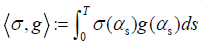note that optimal choice of g for efficient Monte Carlo simulation is achievable, by Section 4, the choice of g such that g(i)=σ(i) for all i∈{1,…, m} minimizes the variance of the weight of Δ. Other Greeks like Γ, vega, ∧ are similarly computed in Subsection 3.2-3.4. Moreover we note that,

i) Given differentiating the payoff function φ inside expectation tends to be easier than our approach applying Malliavin calculus.

ii) In the right-hand of the expression (1), no derivative of the payoff function φ appears any more.

Based on these observations, it is tempted and necessary to relax the restriction of φ. Therefore, by Section 5, we extend the results to a class of non-differentiable payoff functions.

Formulation

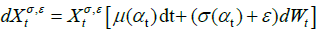
Consider a standard Brownian motion (W_t)_t∈R+ and a Markov chain (α_t) _t∈R+, assume that they are independent and the Markov chain αt has a state space M={1,…, m}.Consider the stochastic process (X_t)_t∈R+ given by the following SDE:

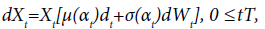(2)

with and and σ: M→(0, ∞), are deterministic functions. Denote the filtration generated by (B_t)_t∈R+ and (α_t)_t∈R+ as (F_t)_t∈R+. Given a payoff function φ on consider t

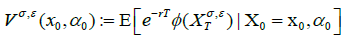
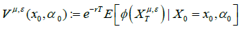
he value function V(x₀, α₀) defined as follows:

(3)

Where (X_t)_t∈[0,T] follows SDE (2), r>0 denotes the risk-free rate. Then we proceed to compute the sensitivities of V(x₀, 0) to the changes of coefficients in this model, such like X₀=x₀, μ, σ and even Q-matrix. To begin with, we recall some Malliavin operators. For any random variable F∈L²(Ω,P) of the form:

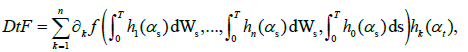
For and deterministic functions h_i: M→R, i∈{0,1,…,n}. Given F∈L²(Ω,P) in the form of (3), the gradient of F is defined by

(4)

For t∈[0,T]. For any deterministic function g : MR we define

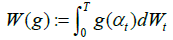(5)

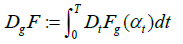(6)

for any random variable F∈L²(Ω,P) in form of (3).

Computation of the Greeks based on the Partial Malliavin Calculus

In this section, we proceed the computation of the sensitivities of V(x₀, 0) to the changes of coefficients in this model, such like X₀, μ, . First in this section, we assume that and has bounded derivative, extension to non-differentiable payoff function will be shown in Section 5.

Variations in the initial price

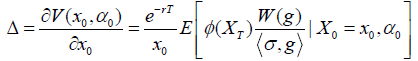
The sensitivity of value function (2) to the initial price X₀ is given by the following proposition:

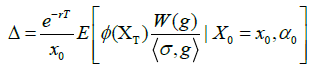
Proposition 3.1 For any payoff function with bounded derivative (X_t)_t∈[0,T], defined in (2) and any g: M→(0,∞), we have

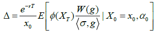
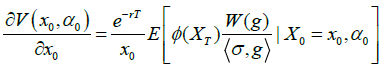(7)

Where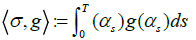

Proof

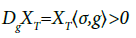
First we check that the right-hand side of (7) is well defined by the following points,

i) 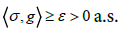for some ε>0, since σ(i)>0 and g(i) > 0 for all iM

ii) We show that 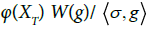is integrable. Since

and Eφ(X_T)²]<∞ for φ is a bounded function, we claim the integrability of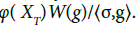

For the left-hand side, we need to show that V(x₀,α₀) is differentiable with respect to x₀. Since φ has bounded derivative, there exists a K₀>0 that 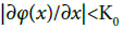for any x∈R. We have the solution to the SDE (2)

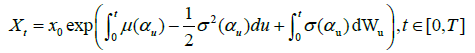(8)

it follows that

which is uniformly bounded by an integrable random variable X_TK₀/x₀.

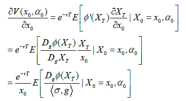
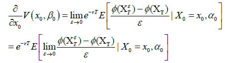
Therefore by V(x₀,α₀) is differentiable with respect to X₀=x₀ and

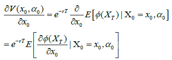(9)

Then we continue to prove (7). It follows from (8) that X_T∈L²(Ω,P) in form of (2), and we have

(10)

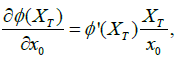
Since the payoff function 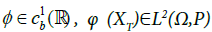and is in form of (2), we have the following chain rule:

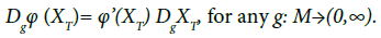(11)

Hence by (8-10) we see that

(12)

Denote by F_α a filtration generated by {α_t; t∈[0,T]}, it follows from the integration by parts formula by Lemma 1.2.1 in Nualart et al. [15] and the independence between (W_t) _t∈[0,T] and (α_t) _t∈[0,T] that,

for any g: M→(0,∞). By (12,13), we obtain,

Variations in the initial price for second order

As in most context, the second derivative of the value function with respect to the initial price is denoted as . Similarly, we have,

Proposition 3.2 For any payoff function with bounded derivative, g: M→(0,∞), and (X_t)_t∈[0,T] defined in (2), we have

Where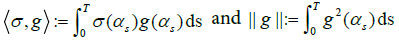

Proof.

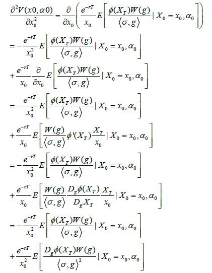(13)

Where a.s. By the chain rule of derivative and the independence between (W_t) _t∈[0,T] and (α_t) _t∈[0,T] we have

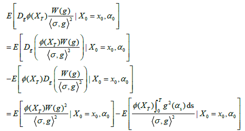(14)

where in the last line we applied the integration by parts formula. Substituting (14) into (13), we see that

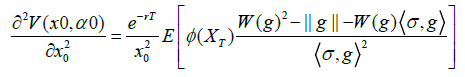
Where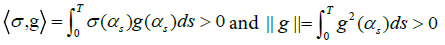

Variations in the diffusion coefficient

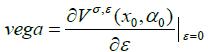
The variations in the diffusion coefficient is denoted as Vega, precisely,

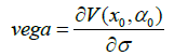
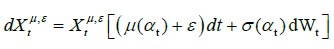
where σ is a constant parameter. In our model, σ(.) is a function on M, so there is no direct way of derivative. Instead, we introduce the perturbed process:

(15)

Where 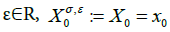Accordingly, we define

(16)

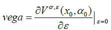
Then the variation in the diffusion coefficient is given by

(17)

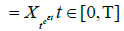
Note that the solution to (15) is

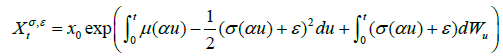
For t∈[0,T], we compute Vega by the following proposition.

Proposition 3.3 For any payoff function with bounded derivative, g: M→(0,∞), and (X_t) _t∈[0,T] defined in (2), we have

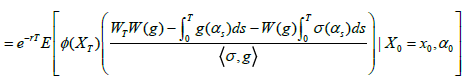(18)

Where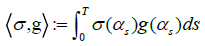

Proof. By the integration by parts formula and chain rule we have,

(19)

for any deterministic function g: M→R, ε∈R. Note by (18) that

the expression Vega in (18) is obtained by passing ε to 0 in (19).

Variations in the drift coefficient

Similarly, we introduce the perturbed process for drift coefficient:

(20)

and the value function driven by

(21)

Accordingly, we have the solution to (20) as follows,

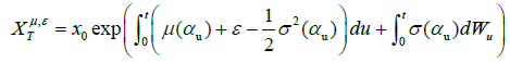(22)

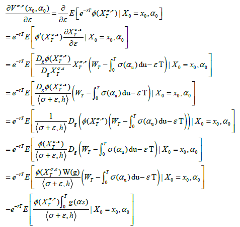
Through a similar computation as that of Vage, we have the derivative of V^μ,ε(x₀,α₀) with respect to ε:

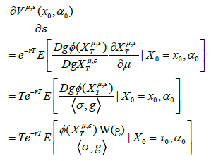
for any deterministic function g : M → R and ε∈R. Therefore, we have the following Proposition 3.4 for Lambda.

Proposition 3.4 For any payoff function with bounded derivative, g: M→(0,∞), and (X_t) _t∈[0,T] defined in (2), we have

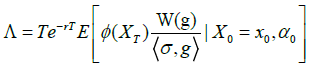
Where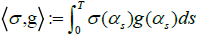

Optimization of Convergence

In this section, we aim at figuring out an optimal choice of g for efficient Monte Carlo simulation. Based on the computation of Theta in a jump diffusion model, Proposition 4.1 of Denis et al. [6] minimizes the variance of the weight of Theta. In our model, there exists such a problem too. We can minimize the weight by choosing a optimal g ∈ G. We gain a similar conclusion to that in Denis et al. [8].

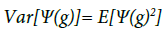
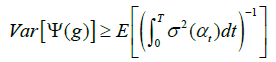
Proposition 4.1 The weight of Delta in (7) is 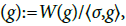then the infimum on {var[Ψ(g)]; g: M→R}is attained when

g(i) = c(i) i ∈M;

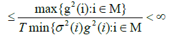
with a constant c > 0, and is given by

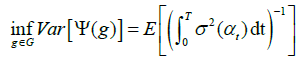
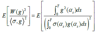
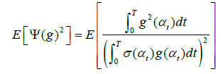
Proof. Since W(g) and , are independent, we have E[Ψ(g)]=0 and

(23)

For any g : M → R, we see that 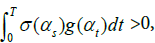with the isometry property of W(g), we have

(24)

By Cauchy-Schwarz inequality,

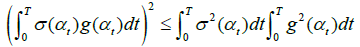
Therefore, by (4.1)-(4.3), we obtain that

In the case of Denis et al. [8], it is proved that the best function chosen in the weight is the constant number. However, in our case, {g(i) = cσ(i) ; i ∈ M} obtains a faster convergence than {g(i) = 1; i ∈ M} does, as shown in the following (Figure 1).

Figure 1: Computation of Delta with respect to the number of samples.

Extension to Non-Differentiable Payoff Function

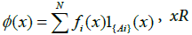
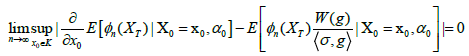
In this section, by a similar arguments as Kawai et al. [16], we show by Proposition 5.1 that the conclusion in Proposition 3.1 below is able to be extended for non-differentiable payoff function in the class ∧(R) defined as in Kawai et al. [16],

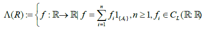
A_i are intervals of R},

Where

Proposition 3.4 For any payoff function with bounded derivative, g: M→(0,∞), and (X_t) _t∈[0,T] defined in (2), we have

(25)

Where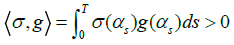

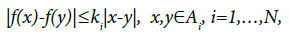
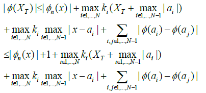
Proof. For any φ∈∧(R), there exists N≥1 and a sequence {k_i∈R₊; i=1,…,N}and a list of disjoint sets (A₁,…,A_N) such that

(26)

where 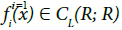with

(27)

And A_i=(a_i-1, a_i], i=1,…,N,

With a₀= -∞ and a_N=∞

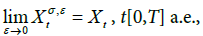
(i) First, we prove that (25) holds for Recalling the definition (2.1) of (X_t) _t∈[0,T], we let X0=x0>0, and for any ε∈R we define by

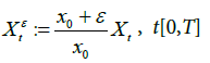(28)

Without letting φ bounded, we can also show that φ(X_T) is integrable. Since φ is continuous, by (27) we see that

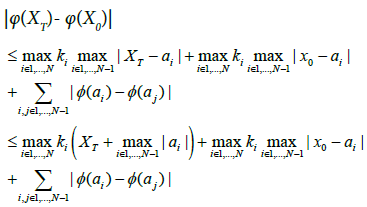
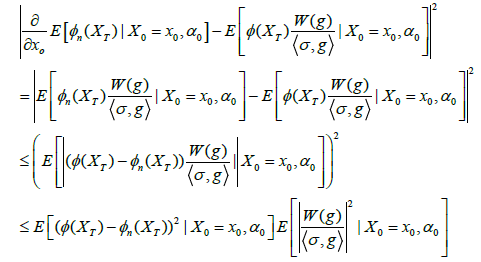
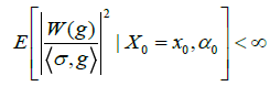
which is integrable, hence the integrability of φ(X_T) is proved. On the other hand, without the bounded derivative of φ, we also show that (10) holds, namely,

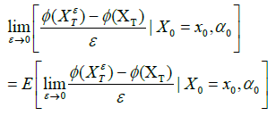(29)

By (27) and definition (28) of X_T^ε we see that

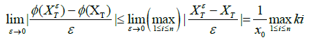
which is uniformly bounded. Therefore, (29) is proved by Lebesgue’s dominated convergence theorem and we have

Relation (26) follows from (31) in the case by repeating the arguments from (10) until the end of Subsection 3.1.

(ii) Finally, we extend from to the class ∧(R). We will structure a sequence approaching to By e.g. Theorem 7.17 of Rudin et al. [17] or (3:6)-(3:7) in Kawai et al. [16], it suffices to show that for all compact set K (0,∞) we have

(31)

for any x₀ ∈ K and

(32)

Since is continuous on every interval (a_i-1, a_i), i=1,…,N, there exists a point wise increasing sequence 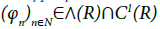such that

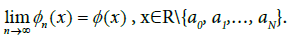(33)

For any 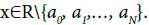there exist such that for n≥N_x we have 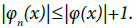Since we see that, for any n≥N_x

which is integrable, hence we can apply the Lebesgue’s dominated convergence theorem and by (34) we obtain (32). Regarding (33), it follows from (i) that (25) holds for any (_n)∧(R)∩C¹(R), therefore

(34)

References

- Fournié E, Lasry JM, Lebuchoux J, Lions PL, Touzi N (1999) Applications of Malliavin calculus to Monte Carlo methods in finance. Fin Stochastics 3: 391-412.
- El-Khatib Y, Privault N (2004) Computations of Greeks in a market with jumps via the Malliavin calculus. Finance and Stochastics 8: 161-179.
- Debelley V, Privault N (Sensitivity analysis of European options in jump discussion models via the Malliavin calculus on the Wiener space Preprint) Sensitivity analysis of European options in jump discussion models via the Malliavin calculus on the Wiener space. Preprint.
- Davis MH, Johansson MP (2006) Malliavin Monte Carlo greeks for jump diffusions. Stoch Process Appl 116: 101-129.
- Bavouzet MP, Messaoud M (2006) Computation of Greeks using Malliavin's calculus in jump type market models. Electron J Probab 11: 276-300.
- Denis L, Nguyen TM (2016) Malliavin calculus for Markov chains using perturbations of time. Stochastics 88: 813-840.
- Bayazit D, Nolder CA (2013) Sensitivities of options via Malliavin calculus: applications to markets of exponential Variance Gamma and Normal Inverse Gaussian processes. Quant Fin 13: 1257-1287.
- Denis L, Nguyen TM (2016) Sensitivities of options via Malliavin calculus: applications to markets of exponential variance Gamma and normal inverse Gaussion processes. Stochastics 88: 813840.
- Liu Y, Privault N (2017) An integration by parts formula in a Markovian regime switching model and application to sensitivity analysis. Stoch Anal Appl 35: 919-940.
- Hamilton JD (1989) A new approach to the economic analysis of nonstationary time series and the business cycle. Econometrica 1: 357-384.
- Yao DD, Zhang Q, Zhou XY (2006) A regime-switching model for European options. In: Stochastic processes, optimization, and control theory: applications in financial engineering, queueing networks, and manufacturing systems. Springer, Boston, USA.
- Kim J, Jeong D, Shin DH (2014) A regime-switching model with the volatility smile for two-asset European options. Automatica 50: 747-755.
- Liu Y, Privault N (2017) A recursive algorithm for optimal selling in regime switching models. Methodol Comput Appl 1702: 1-16.
- Liu Y, Privault N (2017) Selling at the ultimate maximum in a regime-switching model. Int J Theoretical Appl Finance 20: 1750018.
- Nualart D (1995) The Malliavin Calculus and Related Topics. Probability and its Application. Springer, Verlag, USA.
- Kawai R, Takeuchi A (2011) Greeks formulas for an asset price model with Gamma processes. Mathematic Fin 21: 723-742.
- Rudin W (1964) Principles of mathematical analysis. McGraw-hill, New York, USA.