Spanish
  Chinese
  Russian
  German
  French
  Japanese
  Portuguese
  Hindi
Hindi Short Article, Res Rep Math Vol: 2 Issue: 2
Stability of the Stationary Solutions in the Bounded Problem of Eight Bodies with Incomplete Symmetry
Elena Cebotaru*
Technical University of Moldova, Moldova
*Corresponding Author : Elena Cebotaru
Stefan cel Mare si Sfant Boulevard 168, Chisinau 2004, Moldova
Tel: +373 22 237 861
E-mail: elena.cebotaru@mate.utm.md
Received: August 07, 2017 Accepted: March 15, 2018 Published: March 22, 2018
Citation: Cebotaru E (2018) Stability of the Stationary Solutions in the Bounded Problem of Eight Bodies with Incomplete Symmetry. Res Rep Math 2:2
Abstract
It is investigated the stability problem in the Liapunov sense of a new class of exact solutions of the bounded and flat Newtonian problem of several bodies with incompleted symmetry.
Keywords: Stationary solutions; Problem of eight bodies; Liapunov sense
Introduction
It is investigated the stability problem in the Liapunov sense of a new class of exact solutions of the bounded and flat Newtonian problem of several bodies with incompleted symmetry. Whether in the non-coordinate space P0xyz there is the movement of eight bodies P0, P1, P2, P3, P4, P5, P6, P, each having the masses m0, m1, m2, m3, m4, m5, m6, μ, which attract each other in accordance with the law of the universal attraction. We will study the planar dynamic pattern formed by a square in the vertices of which the points P1, P2, P3, P4 are located, the other two points P5, P6, having the masses m5= m6 , are on the diagonal P1P3 of the square at the distances equal to the point P0, in around which this configuration rotates at a constant speed ω determined precisely by the model parameters. The motion of the infinitely small mass μ=0 (the so-called passive gravitational body) will be studied in the gravitational field formed by the seven bodies P0, P1, P2, P3, P4, P5, P6 that attract each other and attract the body P.
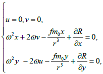
The Liapunov sense of a new class of exact solutions of the restricted and flat Newtonian problem of several bodies with incomplete symmetry is investigated. In the studied model m7=μ=0. For simplicity it will be considered P(x7,y7,z7)≡ P(x,y,z=0) further and then the equations of the point P(x,y,z=0) movement have the form (Figure 1):

Figure 1: Studied model of incomplete symmetry.
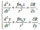 (1)
(1)
where
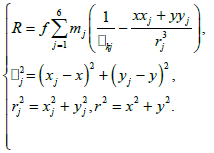 (2)
(2)
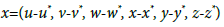
To determine ω them, we will perform such a coordinate transformation that would exclude from the right the equations describing the motion of the bodies during t [1-4]:
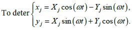 (3)
(3)
Let P1(1,1), P2(-1,1), P3(-1,-1), P4(1,-1), P5(α,α), P6(-α,-α), f=1, m0=1, m5=m6 then, applying the symbolic calculus system Mathematica (SCS Mathematica), we obtain:
 (4)
(4)
The following table shows the tolerable intervals of α it depending on the values of m1 its calculated approximately using the graphical tools of SSC Mathematics (Table 1):
| m1 | Admissible intervals for a |
|---|---|
| 0.0001 | --------------- |
| 0.001 | --------------- |
| 0.01 | (0.8582; 0.85857) |
| 0.1 | (0.715; 0.718) |
| 1 | (0.48965; 0.5053) |
| 10 | (0.291; 0.320) |
| 100 | (0.149; 0.2871) |
| 1000 | (0.050; 0.2838) |
Table 1: According to the definition of the stationary solutions of differential equations, the equilibrium positions (if they exist) are the solutions of the functional equation system.
 (5)
(5)
To determine them, the graphical possibilities of SSC Mathematics were used:To determine them, the graphical possibilities of SCS Mathematica were used:
We will note, for simplicity, the coordinates of any point Ni, Si through  and through the vector
 (6)
(6)
The six-dimensional phase space {x} is local, therefore each of the Ni and Si equilibrium points (taken separately) represents the point x=0 of this space. By performing the linearization procedure in the vicinity of the phase point with SCS Mathematica we obtain the following system of linear differential equations (Table 2):
| m1 | a | N1 | S1 | ||
|---|---|---|---|---|---|
| x* | y* | x* | y* | ||
| 0.01 | 0.8583 | 1.15589 | 1.15589 | 1.39868 | -0.22286 |
| 0.01 | 0.8584 | 1.15597 | 1.15597 | 1.41168 | -0.12379 |
| 0.01 | 0.8585 | 1.15604 | 1.15604 | 1.41684 | -0.05223 |
| 0.01 | 0.85853 | 1.15606 | 1.15606 | 1.41760 | -0.03417 |
| 0.1 | 0.715 | 1.34188 | 1.34188 | 1.34865 | -0.45766 |
| 0.1 | 0.717 | 1.34324 | 1.34324 | 1.44139 | -0.11335 |
| 1 | 0.48965 | 1.63351 | 1.63351 | 0.93934 | -1.05917 |
| 1 | 0.505 | 1.66022 | 1.66022 | 1.82285 | -0.00771 |
| 10 | 0.291 | 1.84521 | 1.84521 | 2.19692 | -0.00052 |
| 100 | 0.2 | 1.82945 | 1.82945 | 0.82914 | -0.02594 |
| 1000 | 0.2 | 1.81083 | 1.81083 | 2.10424 | -0.05038 |
Table 2: Possibilities of SCS Mathematica.
 (7)
(7)
Where the matrix A of the size 6x6 has the form:
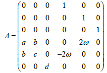 (8)
(8)
For each equilibrium position the values of the elements a, b, c, d of the matrix A will be different. The characteristic equation from which the matrix A’s own values are determined is:
 (9)
(9)
In order for each of the researched equilibrium positions to be stable, it is necessary that all solutions of the equation to be imaginary. As d<0 we obtain that two matrix values A will always be imaginary. We will note them in the future through λ5, λ6 Table 3.
| m1 | a | N1 | S1 | ||
|---|---|---|---|---|---|
| λ1,λ2 | λ3,λ4 | λ1,λ2 | λ3,λ4 | ||
| 0.01 | 0.8583 | ±1.30918 | ±1.12374i | ±0.28434i | ±0.51826i |
| 0.01 | 0.8584 | ±1.30792 | ±1.12295i | ±0.49471i | ±0.32201i |
| 0.01 | 0.8585 | ±1.30666 | ±1.12216i | ±0.45941i | ±0.36935i |
| 0.01 | 0.85853 | ±1.30627 | ±1.12197i | ±0.00440i+0.36926i | ±0.00440-0.36926i |
| 0.1 | 0.715 | ±1.19131 | ±1.06789i | ±0.34443+0.53193i | ±0.34443-0.53193i |
| 0.1 | 0.717 | ±1.17894 | ±1.06051i | ±0.40784+0.56449i | ±0.40784-0.56449i |
| 1 | 0.48965 | ±1.36716 | ±1.30616i | ±0.74472+0.82809i | ±0.74472-0.82809i |
| 1 | 0.505 | ±1.23329 | ±1.12811i | ±0.75807+0.83104i | ±0.75807-0.83104i |
| 10 | 0.291 | ±2.50383 | ±2.63038i | ±1.6617+1.88497i | ±1.6617-1.88497i |
| 100 | 0.2 | ±8.22619 | ±8.56881i | ±15.3124 | ±8.390991i |
| 1000 | 0.2 | ±27.1564 | ±28.0709i | ±17.7615+19.8928i | ±17.7615-19.8928i |
Table 3: Values for stationary points Ni and Si.
Theorem 1
There are values of the parameters m1 and α for which the bisectoral stationary points Si of the boundary problem of eight bodies are stable in the first approximation.
Normalization of the Hamiltonian’s square part
The study of the stability in the Liapunov sense of the stationary points in the fourth order Hamiltonian systems can be made only on the basis of Arnolid-Mozer theorem. In order to verify that the conditions of this theorem are met in the previously studied model, we will first attempt to bring Birkg of into normal form in a series of powers in the vicinity of any stationary point, stable in the first aroximation. In the subsequent calculations and transformations, the stable stationary point was used in the first approximation S1 with the coordinates [5-7].
x*=1.4116760833927924, y*=-0.12379179384743404, (10)
obtained for m1=0.01, α=0.8584, We build, in a rather small neighborhood of this point, the decomposition of Hamiltonian’s series of powers with the accuracy up to the fourth power of the X, Y coordinates and the PX, PY impulses. We will have:
H=H2(X,Y,PX,PY)+H3(X,Y)+H4(X,Y)+R5(X,Y), (11)
Where Hk,(k=2,3,4) there is a homogeneous k-grade, and the R5 rest of the decompose in the Taylor series. For the studied case the square shape and the 3 and 4 forms are equal to:
 (12)
(12)
H3=0.1667(1.4248X3-0.7599X2Y-2.007XY2+0.1931Y3) (13)
H4=0.04167(-4.01396X4+3.7127X3Y+11.6388X2Y2-2.8827XY3- 1.5419Y4) (14)
Berkgof’s theorem on Hamiltonian normalization indicates that first such an un-generated transformation (X,Y,PX,PY)→(p1, p2,q1,q2) should be found that would exclude from H2 the square form the products of impulses and coordinates (p1q1, p2q1, q1q2, q2p1, q2p2, p1p2) and leave only their squares p12 , p22 ,q12 ,q22. In addition, the coefficient of the sum  must be the size
 and the sum
  - the size
 where the λ1,λ3 different values of the matrix are different A. We will look for these transformations in the form of:
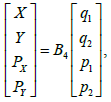 (15)
(15)
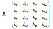
Where B4 is an unknown matrix of size 4×4. The matrix elements, after performing the necessary matrix transformations, are determined from the system of linear equations of the order of 16:
C16z=0 (16)
Where ZT=(b11, b12,…,b44) the vector transposed by the size 16 is made up of the matrix elements
 (17)
(17)
C16 is a matrix of size with known elements. For point S1, a simplex matrix B4 exists and is equal to:
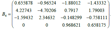 (18)
(18)
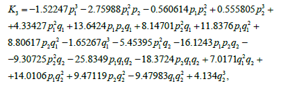
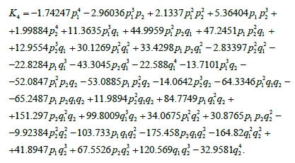
By making the corresponding transformations the forms K2, K3, K4 of Hamiltonian K (written in the new coordinates) will be determined from the relations:

Normalization in Berkgof sense of the cubic form and Hamiltonian’s fourth order form
In order to move to the angles-of-action variables, we will use Berkgof’s classic transformation:
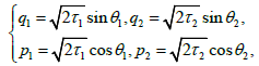 (19)
(19)
where the new variables τ1, τ2, θ1, θ2are angular-action variables. If we write the new Hamiltonian F in the form:
 (20)
(20)
then after performing the corresponding transformations we obtain:
 (21)
(21)
In the vicinity of the stationary point the Hamiltonian equations in the new coordinates are expressed by the formulas:
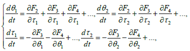 (22)
(22)
The Arnolid-Mozer theorem requires the construction of yet another canonical transformation
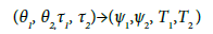 (23)
(23)
which would nullify the third order shape in the Hamiltonian transfomation, and would exclude from the shape of the four phased angles, yet leaving the corresponding square shape F2(τ1,τ2) unchanged.
We will look for this transformation into form:
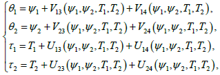 (24)
(24)
where unknown functions V13,V23,U13,U23 are third order shapes, and V14,V24,U14,U24 are fourth order forms with respect to T1,T2.
Performing the transformation (22) by means of the determined functions V13,V23,U13,U23,V14,V24,U14,U24 is obtained for the Hamiltonian W in the vicinity of the stationary point S1 with the coordinates (10), calculated for the m1=0.01 α=0.8584, final form:
 where
where
W2 ( T 1 , T 2) = σ 1T 1- σ 2T 2= 0 . 4 9 4 7 0 7 8 8 4 7 2 4 4 8 2 0 7 T 1 - 0.32200478020850365T2 (25)
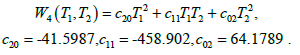 (26)
(26)
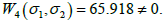
Thus, the purpose of all the above transformations consisted in the fact that after their execution the square W2 and the fourth order W4 depend only on the impulses T1, T2, and the cubic form is canceled. (W3≡0).
Similar results were obtained for the other equilibrium bisectorial positions Si. This result indicates that all the calculations made in SCS Mathematica are correct and consistent with the theoretical conclusions resulting from the symmetry of the studied gravitational model. Thus it can be concluded that stable stationary points in the first approximation are also stable in Liapunov sense [8-12].
Theorem 2
There are values of the parameter m1and corresponding values of the parameter for α which the stationary points of the boundary problem of the eight bodies are stable not only in the first approximation but are also stable in the Liapunov sense.
Conclusion
There are values of the parameters m1 and α for which the bisectoral stationary points Si of the boundary problem of eight bodies are stable in the first approximation and in the Liapunov sense.
References
- Abalakin VC (1971) Reference guide to celestial mechanics and astrodynamics. The science.
- Sebehey V (1982) The theory of orbits, The limited three-body problem. M Science.
- Wintner A (1965) Analytical foundations of celestial mechanics. M Nauka.
- Meyer KR, Schmidt DS (1988) Bifurcations of relative equilibria in the 4-and 5-body problem. Ergod Theory Dyn Syst 8: 215-225.
- Grebenikov EA, Kozak-Skovorodkina D, Yakubyak M (2002) Methods of computer algebra in the problem of many bodies. Publishing house Ros, Russia.
- Vazov V (1968) Asymptotic expansions of solutions of ordinary differential equations.
- Wolfram S (1999) The mathematica. Cambridge: Cambridge university press, India.
- Newton I (1936) Mathematical Principles of Natural Philosophy. Lat AN SSSR.
- Duboshin GN (2002) Celestial Mechanics. Main tasks and methods. Publishing house of Peoples Friendship University, Russia.
- Lagrange IL (1878-1912) Researches on the way of forms of the planets tables by the only obsrevations. Oeuvres, Paris, UK.
- Golubev VG, Grebennikov EA (1985) The problem of three bodies in celestial mechanics. Izd-vo, Moscow University, Russia.
- Elmabsout BA (1987) On the existence of certain configurations of relative equilibrium in the problem of N bodies. Celestial mechanics 41: 131-151.