Research Article, J Nucl Ene Sci Power Generat Technol Vol: 14 Issue: 2
Study of The Indian Energy Consumption in Context to the GDP Growth: Using ARIMA and Factor Analysis
Renuka Devi1*, Alok Agrawal1, Joydip Dhar2 and Sant Pal Singh1
1Department of Applied Sciences, Amity University, Uttar Pradesh, Lucknow, India
2Department of Sciences, Indian Institute of Information Technology and Management, Gwalior, MP, India
*Corresponding Author: Renuka Devi
Department of Applied Sciences, Amity University, Uttar Pradesh, Lucknow, India; E-mail:renuka.niranjan@yahoo.com
Received date: 21 June, 2024, Manuscript No. JNPGT-24-139540;
Editor assigned date: 24 June, 2024, PreQC No. JNPGT-24-139540(PQ);
Reviewed date: 09 July, 2024, QC No. JNPGT-24-139540;
Revised date: 15 April, 2025, Manuscript No. JNPGT-24-139540 (R);
Published date: 22 April, 2025, DOI: 10.4172/2325-9809.1000439
Citation: Devi R, Agrawal A, Dhar J, Singh SP (2025) Study of The Indian Energy Consumption in Context to the GDP Growth: Using ARIMA and Factor Analysis. J Nucl Ene Sci Power Generat Technol 14:2.
Abstract
This research study developed an understanding that there is a converse relationship between GDP growth and energy consumption. Through this study, the authors represented the discussion from an international point of view, then narrowed it to Asia, and finally to the centres in India using the data from secondary sources. The energy consumption data were collected from official sources like government agencies between 1990 and 2019 to maintain authenticity. The authors used two different mathematical approaches to derive the qualitative and quantitative results. The first one was ARIMA (p,d,q), based on the Box-Jenkins methodology. RMSE, AIC, normalized BIC criteria, significance level, R2, etc. were used to identify the best forecasting model. The results show that the four ARIMA models were identical but as per the findings from ARIMA (2,3,8) model was the best forecasting model to predict the Indian GDP growth. The second one was to understand the characteristics of the eight variables, where the factor redemption technique was applied with the help of PCA and the Varimax rotation method. The KMO and Bartlett’s tests were applied for the measurement of sampling adequacy and sphericity as two different approaches. In this research work, authors studied the different parameters like AIC, Normalized BIC method, RMSE, MSE, t-test, and significance level method to find out the best suitable ARIMA model for the Indian GDP growth.
Keywords: ARIMA; Time series; Box-L Jung; Gross domestic products; Energy consumption
Introduction
The energy consumption and quality of life are connected directly. If humanity has access to clean, safe, secure, affordable, and abundant energy, then it would be so much beneficial. Simultaneously extraction, transportation, and use of energy can adversely affect the health, environment, and economy. As of today, every nation is not self-sustainable in energy production, so reliance on imported energy can create national security vulnerabilities. The position of the Asia Pacific region is lower than that of Western countries in the context of energy production and consumption [1]. The regional electrification rate reached 96.6% with great progress in previous decades. The number of people lacking an electric connection has dropped from 545 million to 157 million between 2010 to 2019 despite continuous population growth. India is a country where the population and economy are growing simultaneously, thus it has increased power consumption. The power demand is expected to increase at an annual rate of 6.5% between 2020 to 2024 as projected by the International Energy Agency (IEA) per the current behavior of industrial and residential consumption. During the COVID-19 pandemic, the energy demand declined by 7%, but by June 2021 it again got shot up to around 10%, which also resulted in a temporary coal shortage [2]. India is also moving towards the adoption of electric vehicles. This could be one of the many examples which will surely boost the power consumption of both domestic and commercial types. Thus, the production of electricity in India still depends majorly on thermal and hydropower plants. India has been involved in nuclear, solar, wind, etc. type of other sources, but all those require innovation and investments.
Energy consumption is a prime topic for the researcher. China, Turkey, and other countries are also concerned about the production and consumption pattern of energy. The sources of energy (coal, oil, natural gases, etc.) are correlated with environmental quality [3-5]. Indian GDP is always a highlighted topic for researchers and the relation of GDP growth and energy consumption are related to each other. This kind of literature tried to highlight the importance of GDP calculation and analyse the different techniques of GDP forecasting. Residential energy consumption of the household sector in countries belonging to the Euro area. In this research, researchers have applied the accuracy model between three different models (0,1,1), (1,1,0), and (1,1,2) and find out the best model based on RMSE and MAE results. Researchers find out that ARIMA (0,1,1) model provided a more accurate result rather than the other models. The main focus of this research is how non-CO2 activities will be performed in the future to protect the environment and how we can improve the consumption of renewable energy sources [6]. Other research works that will help to understand the role of multivariate time series. A multivariate time series model is used to forecast future electricity usage. Researchers have applied three different methods like ARIMA, LSTM, and RNN to forecast the actual future consumption of energy. The prediction period of results was classified based on three categories: Short-term, mid-term, and long-term. In this research, the study was conducted to predict individual and block energy consumption and the comparison of results based on these different methods [7].
The consumption of energy in two different situations i.e., precovid and during covid pandemic in the United State. The United States is known as the second-highest energy consuming country in the world. During the pandemic the whole world has faced different types of challenges, even the U.S. economy was not only affected by the trade but also the decline rate in energy consumption. To understand future growth in energy consumption, the researchers have applied the ARIMA and ARIMA-BP techniques. To develop an accurate future predicted model researchers have used the Mean Absolute percentage error and applied the combination principle that is known as ‘error correction + secondary modeling’ to conduct the combined research on individual ARIMA and ARIMA-BP models. The accuracy of results was higher in both ARIMA (94.4%) and ARIMA-BP (95.4%), which represented that the combined principle was the best technique to predict future energy consumption [8]. A small-scale data set and the Internet of Things was used to collect the dataset. There is other research, where five different types of analysis models (ARIMA, ARIMA-GBR, ARIMA-SVR, LSTM, and GRU) were applied. Researchers have find-out that the ARIMA-SVR model was the best-fitted model among all. The accuracy and credibility of this model are based on the MSE, MAPE, and RMSE results [9, 10].
The electrical load and the ARIMA methods are used to forecast the value of the electrical load. This research work helped to shape the energy policy and the power system sustainability. In this research, the authors considered two additional phases in the standard ARIMA model, these two phases are identification of noise level and signal fettering. India is the second largest populated country, so the consumption of energy is increasing day by day. In this research, authors have tried to forecast the energy consumption demand by 2030. For this analysis, two different groups of power plants: one is a coal and lignite-based power plant, and the second one is a renewable energy-based plant. This study will be helpful to understand the future demand for renewable energy.
Indian GDP growth is related to the primary, secondary, and territory sectors. Energy production and consumption are equally important factors in Indian economic growth. Researchers have developed the bond between economy and energy consumption by applying different methods. Factor analysis is one of the techniques that has been applied in this research work. The different dimensions of energy consumption and production are explained by the authors. The correlation between electricity consumption and consumer income. This study also talks about the use effectiveness of alternate energy in the domestic sector. Important points like the use of renewable energy in the domestic sector and the replacement of fossil fuel with solar energy are introduced. To analyze the historical movement of the Indian economy in view of recent up and downs and thereby also forecast the future economic movement by using the time series as the statistical tool. The prime objective is to explore the relationship between electricity consumption, trade openness, and economic growth in India. For this purpose, the co-integration test and Granger causality vector error correlation model are essential. This specific research work is based on understanding the possible relationship between energy production and GDP growth. That explores the causality between various variables which have great application in the field of climate change and sustainable development.
Materials and Methods
Mathematical description
This research work is focused on time series analysis. There are different methods to forecast the value. There are different types of literature, that the researcher tried to highlight in the literature work. Based on research work, the ARIMA method is more accurate and simpler to predict the values. So, researchers have referred to the ARIMA modeling method to forecast the Indian GDP values. This research work is based on two different statistical techniques, ARIMA and Factor analysis method.
Autoregressive Integrated Moving Average (ARIMA)
ARIMA modeling process passed through three stages i.e., identification, estimation, and diagnostic checking. The ARMA (Autoregressive moving average) is the combination of two polynomial AR and MA. AR stands autoregressive and MA stands moving average. The ARIMA model is represented by (p,d,q).
Mathematical description of the regression analysis model
The Autoregression analysis (AR) at order ‘p’ process is:

If we have AR(p), â??pâ?? number of past values then

The process of the MA model for order â??qâ?? is

If we have MA(q), â??qâ?? number of past values then

The ARMA (p, q) model is:

Mathematical description of factor analysis method
Factor analysis is a factor redemption technique that permits a large number of interrelated variables to a smaller number of common factors that can explain the maximum variance in the original set of variables.
The matrix model of the factor analysis method is

The general format of the factor analysis method is
x-μ=αF+p
Results and Discussion
Formulation and implementation of model
This research work is based on the Indian current GDP structure. To understand the gravity of GDP in society and economy researchers have collected the GDP and consumption data. The Data is based on the current US $ Yearly and to understand the microstructure of the data, data is interpolated yearly to quarterly by using the Denton method. And all the other consumption variables also change on the basis of requirements. The data is collected from the BP Oil industry company, London, England government website and the duration of data is 1990Q1 to 2019Q2 . So, the total number of observations is 116 and the Excel and SPSS software were applied.
The details of consumption variables are as follows:
x1=Electric power consumption
x2=Oil consumption
x3=Natural gas consumption
x4=Coal consumption
x5=Nuclear energy consumption
x6=Hydroelectricity consumption
x7=Consumption of fixed capital (adjusted savings current US $)
x8=Household and NPISHs final consumption expenditure PPP
x9=GDP (current US $)
Energy consumption in India is growing too fast and the details of the growth rate can be represented by the graph.
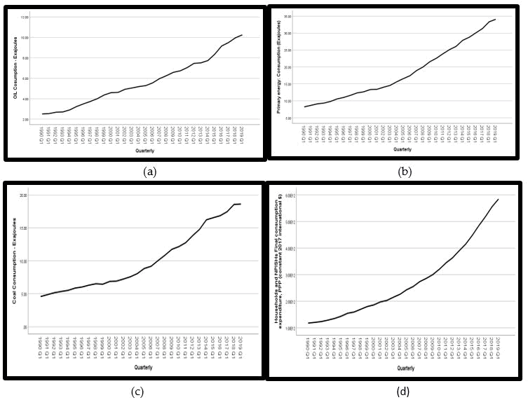
Figure 1 shows that oil consumption, primary energy consumption, coal consumption, and household and NPISH consumption variables have smooth growth with respect to time. Figure (a) shows that the growth rate from 1993Q1 to 2019Q1 has tremendous growth. And figure (b) primary energy has shown smooth linear growth. The primary energy consumption in 1990Q1 is around 8.0 exajoules and in 2019Q1 it reached 34 exajoules. Figure (c) represented the coal consumption growth, 1990Q1 growth is 4.9 exajoules, and after 10 years from 2000Q1 to 2010Q1 , it touched the growth rate from 7 exajoules to 13 exajoules. After comparing Figures (a) and Figure (c), it is clear that coal consumption is greater than oil consumption growth. Figure (d) shows the positive household and NPISH consumption growth rate. Figure (d) represented that from 1990Q1 to 200Q1 the growth rate is not as high as from 2001Q1 to 2010Q1 and from 2010Q1 household and NPISH consumption is 3.00 E+12 and in 2019Q1 it reached 5.9 E+12.
Figure 1: (a-d): Graphical presentations of consumption variables like primary energy, oil, coal, and household consumption.
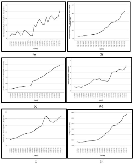
Figure 2 represented the growth rate of six variables like hydroelectricity consumption, consumption of fixed capital, electric power consumption, nuclear energy consumption, natural gas consumption, and GDP variables but the growth of these variables is not as smooth as the Figure 1 variable with respect to time. Figure (e) shows the hydroelectricity consumption growth from 1990Q1 to 2019Q1 , this Figure (e) represented that from 1990Q1 to 1998Q1 the growth rate is very slow and there are many ups and downs. From 1998Q1 the growth line starts decreasing suddenly but after 2003Q1 there is a high positive growth rate in just one year (2004Q1).
Figure (f) represented the growth rate of consumption of fixed capital and this figure shows that there are not many ups and downs and the growth rate is moving towards an upward direction and maintained a continuous growth rate. Figure (g) represented the electricity consumption growth rate which is the most common consumption energy source in India. From 1990Q1 to 2002Q1, the electricity growth is very slow but after that in 2003Q1, there is a boom in electricity consumption. In the next 15 years, the growth rate is reached from 600 kwh to 1200 kwh per capita consumption rate.
Nuclear energy sources are very popular energy sources all over the world. Figure (h) nuclear energy consumption rate is very slow in India in 1990Q1. Their growth rate graph represented that there is a sudden growth in nuclear consumption in 1997Q1 and 2009Q1 but compared to the other variables growth rate is not as positive as the others. Figure (i) natural gas consumption graph shows that from 1990Q1 to 2007Q1 growth moved smoothly with respect to time but after 3 years in 2010Q1 it touched the highest consumption point. After that, the growth starts decreasing in 2019Q1 and the growth rate is the same as in 2010Q1. Figure (j) represented the economic growth (GDP) of India. GDP is the dependent variable in this research work. And the graph of GDP shows that from 1990Q1 to 2002Q1 the growth rate is very smooth but after that from 2003Q1 to 2019Q1 there is a high positive growth rate.
Figure 2: (e-j): Graphical presentations of variables like hydroelectricity, consumption of fixed capital, electric power, nuclear energy, natural gas, and GDP.
Autoregressive Integrated Moving Average (ARIMA)
To understand the pattern of consumption and forecast the consumption of the future, an ARIMA method is a suitable statistical time series technique. ARIMA is the most suitable method to forecast the future value with accuracy and this method is not only suitable for energy consumption but also for other sectors. An ARIMA is a model that is based on past data to predict future values. To predict future values, the data should be stationary. Stationary time series is one where the means and variance are constant over time. To transform the non-stationary time series into a stationary time series the differencing method is applied. Figure 1 and 2 is representing the non-stationary time series values (d=0).
Autocorrelation and partial autocorrelation function
ACF and PACF method is used to predict the ‘AR’ and ‘MA’ values. An ACF value is useful to determine, how correlated a time series is with its past values. And PACF is a summary of the relationship between an observation in a time series with observations at prior time steps with the relationship of intervening observations removed. Figure 2 is representing the ACF and PACF values with lag values.
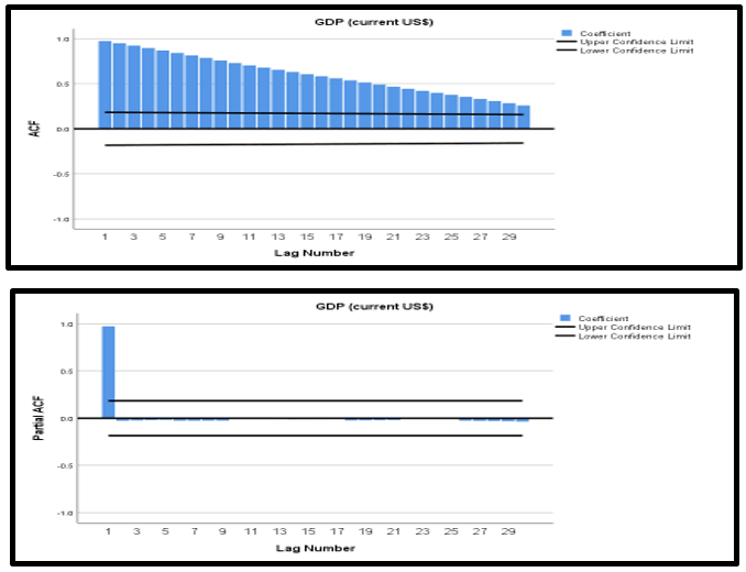
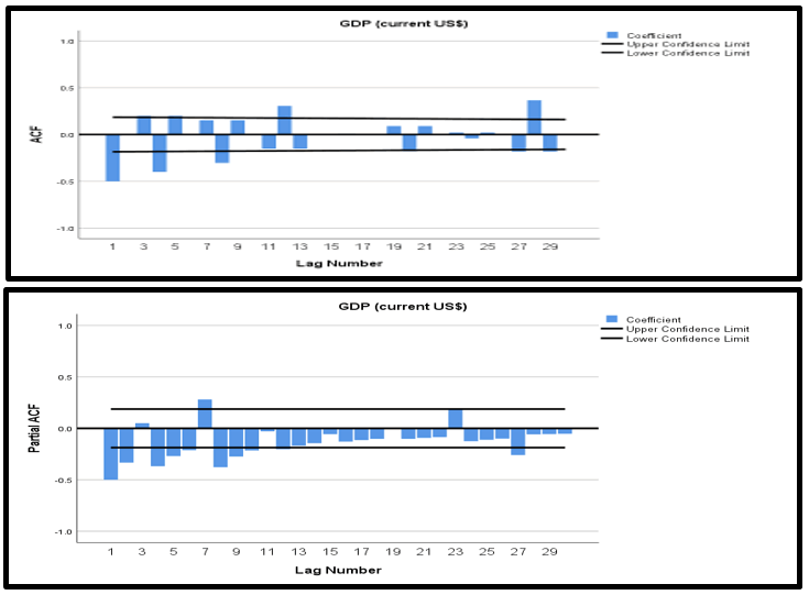
Table 1 and Figure 3 have been representing that the time series data is non-stationary. So, the next step is to transform the time series from non-stationary to stationary by using the difference method. Table 2 and Figure 4 represent the difference data series. Here the value of d is 3.
| Series: GDP (current US $) | |||||||
| Autocorrelations | Partial autocorrelations | ||||||
| Lag | Autocorrelation | Standard errora | Box-Ljung statistic | Partial autocorrelations | Standard error | ||
| Value | df. | Sig. b | |||||
| 1 | 0.975 | 0.091 | 114.084 | 1 | 0 | 0.975 | 0.092 |
| 2 | 0.949 | 0.091 | 223.166 | 2 | 0 | -0.026 | 0.092 |
| 3 | 0.923 | 0.09 | 327.214 | 3 | 0 | -0.023 | 0.092 |
| 4 | 0.897 | 0.09 | 426.244 | 4 | 0 | -0.019 | 0.092 |
| 5 | 0.87 | 0.09 | 520.321 | 5 | 0 | -0.016 | 0.092 |
| 6 | 0.843 | 0.089 | 609.412 | 6 | 0 | -0.026 | 0.092 |
| 7 | 0.815 | 0.089 | 693.499 | 7 | 0 | -0.025 | 0.092 |
| 8 | 0.787 | 0.088 | 772.583 | 8 | 0 | -0.025 | 0.092 |
| 9 | 0.758 | 0.088 | 846.68 | 9 | 0 | -0.025 | 0.092 |
| 10 | 0.731 | 0.088 | 916.134 | 10 | 0 | 0.008 | 0.092 |
| 11 | 0.704 | 0.087 | 981.264 | 11 | 0 | 0.007 | 0.092 |
| 12 | 0.679 | 0.087 | 1042.371 | 12 | 0 | 0.006 | 0.092 |
| 13 | 0.655 | 0.086 | 1099.733 | 13 | 0 | 0.006 | 0.092 |
| 14 | 0.631 | 0.086 | 1153.49 | 14 | 0 | -0.009 | 0.092 |
| 15 | 0.607 | 0.086 | 1203.786 | 15 | 0 | -0.009 | 0.092 |
| 16 | 0.584 | 0.085 | 1250.769 | 16 | 0 | -0.008 | 0.092 |
| 17 | 0.561 | 0.085 | 1294.595 | 17 | 0 | -0.008 | 0.092 |
| 18 | 0.538 | 0.084 | 1335.3 | 18 | 0 | -0.023 | 0.092 |
| 19 | 0.515 | 0.084 | 1372.937 | 19 | 0 | -0.021 | 0.092 |
| 20 | 0.491 | 0.083 | 1407.567 | 20 | 0 | -0.02 | 0.092 |
| 21 | 0.467 | 0.083 | 1437.263 | 21 | 0 | -0.019 | 0.092 |
| 22 | 0.444 | 0.083 | 1468.19 | 22 | 0 | -0.005 | 0.092 |
| 23 | 0.422 | 0.082 | 1494.506 | 23 | 0 | -0.006 | 0.092 |
| 24 | 0.399 | 0.082 | 1518.365 | 24 | 0 | -0.006 | 0.092 |
| 25 | 0.377 | 0.081 | 1539.914 | 25 | 0 | -0.006 | 0.092 |
| 26 | 0.355 | 0.081 | 1559.191 | 26 | 0 | -0.025 | 0.092 |
| 27 | 0.332 | 0.08 | 1576.245 | 27 | 0 | -0.028 | 0.092 |
| 28 | 0.308 | 0.08 | 1591.129 | 28 | 0 | -0.03 | 0.092 |
| 29 | 0.284 | 0.08 | 1603.912 | 29 | 0 | -0.032 | 0.092 |
| 30 | 0.259 | 0.079 | 1614.667 | 30 | 0 | -0.036 | 0.092 |
| Note: a. The underlying process assumed is independence (white noise); b. Based on the asymptotic chi-square approximation. | |||||||
Table 1: Tabulation and representation of ACF and PACF without difference (d=0).
Figure 3: Graphical presentation of ACF and PACF (When d=0).
Figure 4: Graphical presentation of ACF and PACF (When d=3).
| Series: GDP (current US $) | |||||||
| Autocorrelations | Partial autocorrelations | ||||||
| Lag | Autocorrelation | Standard errora | Box-Ljung statistic | Partial autocorrelations | Standard error | ||
| Value | df. | Sig.b | |||||
| 1 | -0.5 | 0.092 | 29.257 | 1 | 0 | -0.5 | 0.094 |
| 2 | 0 | 0.092 | 29.257 | 2 | 0 | -0.333 | 0.094 |
| 3 | 0.2 | 0.092 | 34.03 | 3 | 0 | 0.05 | 0.094 |
| 4 | -0.4 | 0.091 | 53.299 | 4 | 0 | -0.369 | 0.094 |
| 5 | 0.2 | 0.091 | 58.16 | 5 | 0 | -0.269 | 0.094 |
| 6 | 0 | 0.09 | 58.16 | 6 | 0 | -0.212 | 0.094 |
| 7 | 0.152 | 0.09 | 61.012 | 7 | 0 | 0.281 | 0.094 |
| 8 | -0.304 | 0.09 | 72.526 | 8 | 0 | -0.378 | 0.094 |
| 9 | 0.152 | 0.089 | 75.432 | 9 | 0 | -0.274 | 0.094 |
| 10 | 0 | 0.089 | 75.432 | 10 | 0 | -0.215 | 0.094 |
| 11 | -0.153 | 0.088 | 78.426 | 11 | 0 | -0.029 | 0.094 |
| 12 | 0.305 | 0.088 | 90.519 | 12 | 0 | -0.203 | 0.094 |
| 13 | -0.153 | 0.087 | 93.572 | 13 | 0 | -0.169 | 0.094 |
| 14 | 0 | 0.087 | 93.572 | 14 | 0 | -0.144 | 0.094 |
| 15 | -0.004 | 0.087 | 93.574 | 15 | 0 | -0.057 | 0.094 |
| 16 | 0.009 | 0.086 | 93.585 | 16 | 0 | -0.129 | 0.094 |
| 17 | -0.004 | 0.086 | 93.587 | 17 | 0 | -0.114 | 0.094 |
| 18 | 0 | 0.085 | 93.587 | 18 | 0 | -0.102 | 0.094 |
| 19 | 0.09 | 0.085 | 94.709 | 19 | 0 | 0.001 | 0.094 |
| 20 | -0.18 | 0.084 | 99.244 | 20 | 0 | -0.103 | 0.094 |
| 21 | 0.09 | 0.084 | 100.39 | 21 | 0 | -0.093 | 0.094 |
| 22 | 0 | 0.083 | 100.39 | 22 | 0 | -0.085 | 0.094 |
| 23 | 0.021 | 0.083 | 100.455 | 23 | 0 | 0.192 | 0.094 |
| 24 | -0.042 | 0.082 | 100.716 | 24 | 0 | -0.125 | 0.094 |
| 25 | 0.021 | 0.082 | 100.782 | 25 | 0 | -0.112 | 0.094 |
| 26 | 0 | 0.082 | 100.782 | 26 | 0 | -0.1 | 0.094 |
| 27 | -0.183 | 0.081 | 105.856 | 27 | 0 | -0.259 | 0.094 |
| 28 | 0.365 | 0.081 | 126.387 | 28 | 0 | -0.059 | 0.094 |
| 29 | -0.183 | 0.08 | 131.58 | 29 | 0 | -0.056 | 0.094 |
| 30 | 0 | 0.08 | 131.58 | 30 | 0 | -0.053 | 0.094 |
| Note: a. The underlying process assumed is independence (white noise). b. Based on the asymptotic chi-square approximation. | |||||||
Table 2: Tabulation and representation of ACF and PACF with difference (d=3).
To find out the best suitable AR and MA value the Box-Ljung statistic method is applied based on the asymptotic chi-square approximation. After taking the first and second differences the data was not stationary because the spikes are not clear but in Table 2 and Figure 4, the difference 3 is transforming the non-stationary time series to stationary. And the image of spikes is clear which will help us to identify the ‘p’ and ‘q’ values in ACF and PACF. But other differences (d=4, d=5, d=6) are not appropriate because spikes are very small and tend towards 0. It is clear that in difference 3, most of the spikes are between +0.5 to -0.5 confidence levels. After transforming the time series data, the next step is to find out the appropriate ‘p’ and ‘q’ values to decide which will be the best model fitted for this research purpose.
Autoregressive integrated moving average statistical method
To understand the nature of time series data and to forecast the future value calculation, there are several models but the researchers’ task is to find the best fitted model for energy consumption and other factors. ARIMA statistical model will help to identify the best-fitted model. Normalized BIC and Ljung-Box techniques were applied to identify the ARIMA model.
Table 3 represents the combination of different ARIMA models basis on p, d, and q for energy, consumption, and GDP time series data. This table has shown the differences between 3,4,5 and 6 based on the different p and q values and insisted of d=3 other would have higher normalized BIC and RMSE values. This explains that difference 3 is the suitable difference for the ARIMA parameter. Table 3 result explains that the lowest normalized BIC values and lowest RMSE will be helpful to decide the good ARIMA model.
| Model (p,d,q) | Stationary R2 | R2 | RMSE | MAPE | MAE | Max APE | Max AE | Normalized BIC | Ljung Box Q (18) | ||
| Statistics | df | Sig. | |||||||||
| 2,3,8 | 0.705 | 1 | 1.2510 | 0.665 | 5.74 E+09 | 6.279 | 5.59 E+10 | 46.95 | 13.46 | 8 | 0.097 |
| 4,3,8 | 0.714 | 1 | 1.24 E+10 | 0.689 | 6.03 E+09 | 6.279 | 4.94 E+10 | 47.023 | 11.274 | 6 | 0.08 |
| 8,3,1 | 0.723 | 1 | 1.20 E+10 | 0.649 | 5.29 E+09 | 6.581 | 5.03 E+10 | 46.835 | 5.23 | 9 | 0.814 |
| 9,3,1 | 0.723 | 1 | 1.21 E+10 | 0.651 | 5.31 E+09 | 6.849 | 5.03 E+10 | 46.886 | 5.258 | 8 | 0.73 |
| 9,3,3 | 0.726 | 1 | 1.21 E+10 | 0.668 | 5.52 E+09 | 6.818 | 4.82 E+10 | 46.979 | 4.44 | 6 | 0.617 |
| 1,4,7 | 0.88 | 1 | 1.37 E+10 | 0.856 | 7.65 E+09 | 6.279 | 5.54 E+10 | 47.055 | 17.251 | 10 | 0.069 |
| 2,4,5 | 0.869 | 1 | 1.43 E+10 | 0.911 | 8.5 E+09 | 6.279 | 5.79 E+10 | 47.096 | 23.314 | 11 | 0.016 |
| 2,4,8 | 0.884 | 1 | 1.36 E+10 | 0.82 | 7.34 E+09 | 6.279 | 5.38 E+10 | 47.127 | 14.808 | 8 | 0.063 |
| 2,4,9 | 0.893 | 1 | 1.32 E+10 | 0.788 | 6.72 E+09 | 6.279 | 5.39 E+10 | 47.102 | 10.681 | 7 | 0.153 |
| 4,4,5 | 0.879 | 1 | 1.39 E+10 | 0.85 | 7.71 E+09 | 6.279 | 5.52 E+10 | 47.122 | 18.517 | 9 | 0.03 |
| 1,5,6 | 0.938 | 1 | 1.79 E+10 | 1.165 | 1.12 E+10 | 14.017 | 5.59 E+10 | 47.556 | 37.832 | 11 | 0 |
| 1,5,9 | 0.949 | 1 | 1.66 E+10 | 1.108 | 9.98 E+09 | 14.049 | 5.67 E+10 | 47.528 | 25.633 | 8 | 0.001 |
| 3,5,6 | 0.94 | 1 | 1.79 E+10 | 1.25 | 1.16 E+10 | 14.097 | 5.90 E+10 | 47.365 | 29.245 | 9 | 0.001 |
| 3,5,11 | 0.958 | 1 | 1.53 E+10 | 1.073 | 8.89 E+09 | 14.118 | 5.71 E+10 | 47.533 | 11.958 | 4 | 0.018 |
| 6,5,6 | 0.955 | 1 | 1.57 E+10 | 1.162 | 1 E+10 | 14.01 | 4.77 E+10 | 47.503 | 11.423 | 6 | 0.076 |
| 1,6,7 | 0.965 | 0.99 | 2.54 E+10 | 2.142 | 1.74 E+10 | 24.557 | 6.86 E+10 | 48.297 | 17.205 | 10 | 0.07 |
| 1,6,8 | 0.964 | 0.99 | 2.58 E+10 | 2.102 | 1.69 E+10 | 24.557 | 7.51 E+10 | 48.373 | 21.927 | 9 | 0.009 |
| 2,6,8 | 0.965 | 0.99 | 2.55 E+10 | 2.155 | 1.74 E+10 | 24.557 | 6.86 E+10 | 48.388 | 17.156 | 8 | 0.029 |
| 6,6,1 | 0.959 | 0.99 | 2.74 E+10 | 2.447 | 1.90 E+10 | 24.557 | 9.85 E+10 | 48.403 | 16.041 | 11 | 0.14 |
| 6,6,2 | 0.961 | 0.99 | 2.67 E+10 | 2.323 | 1.83 E+10 | 24.557 | 9.56 E+10 | 48.396 | 11.641 | 10 | 0.31 |
Table 3: Representation of combination of different statistical models.
Here, model (8,3,1) normalized BIC value and RMSE value are the lowest 46.835 and 1.202 E+10 respectively among the other models. On the basis of the above calculation the best-fitted models are (2,3,8), (4,3,8), (8,3,1), and (9,3,1). The next step is to select the better-fitted model out of these four good models with the help of the ARIMA parameters. Here, Table 4 shows the outcomes of the ARIMA model.
| GDP (Current US $) | Model | Estimated | S.E. | T | Sig. | |
| Model-1 | ARIMA (2,3,8) | Constant | -7.94 E-05 | 8657192 | -9.17 E-12 | 1 |
| AR (1) | -0.768 | 5.742 | -0.134 | 0.894 | ||
| AR (2) | -0.399 | 4.72 | -0.084 | 0.933 | ||
| MA (1) | 0.249 | 5.755 | 0.043 | 0.966 | ||
| MA (2) | 0.405 | 3.475 | 0.117 | 0.907 | ||
| MA (3) | 0.413 | 4.925 | 0.084 | 0.933 | ||
| MA (4) | 0.79 | 0.134 | 5.873 | 0 | ||
| MA (5) | -0.225 | 4.444 | -0.051 | 0.96 | ||
| MA (6) | -0.322 | 2.813 | -0.114 | 0.909 | ||
| MA (7) | -0.305 | 3.89 | -0.078 | 0.938 | ||
| MA (8) | -0.012 | 0.155 | -0.075 | 0.94 | ||
| Model-2 | ARIMA (4,3,8) | Constant | -7.94 E-05 | 8021015 | -9.90 E-12 | 1 |
| AR (1) | -1.239 | 2.728 | -0.454 | 0.651 | ||
| AR (2) | -0.667 | 3.697 | -0.18 | 0.857 | ||
| AR (3) | 0.078 | 2.185 | 0.036 | 0.972 | ||
| AR (4) | -0.057 | 0.191 | -0.297 | 0.767 | ||
| MA (1) | -0.218 | 3.954 | -0.055 | 0.956 | ||
| MA (2) | 0.624 | 2.683 | 0.233 | 0.817 | ||
| MA (3) | 0.831 | 1.325 | 0.627 | 0.532 | ||
| MA (4) | 0.608 | 2.761 | 0.22 | 0.826 | ||
| MA (5) | 0.268 | 3.006 | 0.089 | 0.929 | ||
| MA (6) | -0.458 | 2.506 | -0.183 | 0.855 | ||
| MA (7) | -0.756 | 1.042 | -0.726 | 0.47 | ||
| MA (8) | 0.09 | 2.305 | 0.036 | 0.969 | ||
| Model-3 | ARIMA (8,3,1) | Constant | -7.94 E-05 | 17369055 | -4.57 E-12 | 1 |
| AR (1) | 0.012 | 0.08 | 0.155 | 0.877 | ||
| AR (2) | 0.012 | 0.08 | 0.144 | 0.886 | ||
| AR (3) | 0.011 | 0.08 | 0.135 | 0.893 | ||
| AR (4) | -0.607 | 0.08 | -7.585 | 0 | ||
| AR (5) | 0.012 | 0.081 | 0.154 | 0.878 | ||
| AR (6) | 0.012 | 0.081 | 0.144 | 0.886 | ||
| AR (7) | 0.011 | 0.081 | 0.135 | 0.893 | ||
| AR (8) | -0.618 | 0.09 | -6.837 | 0 | ||
| MA (1) | 0.996 | 0.323 | 3.082 | 0.003 | ||
| Model-4 | ARIMA (9,3,1) | Constant | -7.94 E-05 | 17797753 | -4.46 E-12 | 1 |
| AR (1) | 0.025 | 0.106 | 0.237 | 0.813 | ||
| AR (2) | 0.011 | 0.081 | 0.139 | 0.89 | ||
| AR (3) | 0.011 | 0.08 | 0.133 | 0.894 | ||
| AR (4) | -0.607 | 0.081 | -7.519 | 0 | ||
| AR (5) | 0.025 | 0.108 | 0.234 | 0.815 | ||
| AR (6) | 0.011 | 0.082 | 0.14 | 0.889 | ||
| AR (7) | 0.011 | 0.081 | 0.134 | 0.894 | ||
| AR (8) | -0.618 | 0.091 | -6.779 | 0 | ||
| AR (9) | 0.021 | 0.119 | 0.18 | 0.858 | ||
| MA (1) | 0.998 | 0.556 | 1.794 | 0.076 |
Table 4: Representation of ARIMA parameters.
There are multiple factors that will help to find the best-fitted ARIMA model. In Table 3, there are four possible outcomes but the picture was not clear because the parameters like RMSE, normalized BIC, R2 , MAPE, MAE, and Ljung Box method are not sufficient to decide which one is suitable for the research. So, ARIMA parameters are based on significance level, t-value, and standard error, these are other characteristics to choose the better-fitted model of time series. Table 4 represented that, the AR (2), AR (4), AR (8), and AR (9) significance levels are 93%, 76%, 00%, and 85% respectively. So, the highest significance level is AR (2) at 93%, and MA (8), MA (8), MA (1), and MA (1) significance levels are 94%, 96%, 00%, and 7%. Between (2,3,8) and (4,3,8) the best-fitted model is ARIMA (p,d,q) (2,3,8) on the basis of significance level and t-value (<0.05) parameters.
ACF and PACF Graph for ARIMA (2,3,8) model
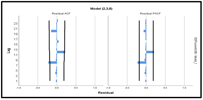
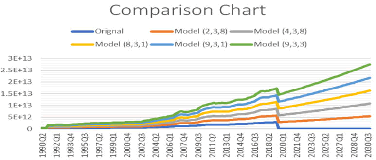
Figure 5 is representing the outcome of ACF and PACF of the ARIMA model (2,3,8). And fitted model of time series. Figure 6 is representing the outcome of all models with the original value.
Figure 5: ACF and PACF for ARIMA (2,3,8) model.
Figure 6: Forecasted values and original value of GDP.
Factor analysis method
Factor analysis is a factor redemption technique (analyzing only common variables). To analyse economic growth, the simplification of parameters is required in factor analysis. In this research paper, the researcher applied the Factor analysis method to categorize the nature of the other variable. But before applying the factor analysis the first step is to create the correlation matrix. The correlation matrix will try to develop the relationship between the variable.
Here, Table 5 is representing the correlation between these system variables. The result shows that all eight variables have a strong and positive correlation with each other (r> +0.9).
| Correlation matrixa | |||||||||
| Electric power con. | Oil con. | Natural gas con. | Coal con. | Nuclear energy con. | Hydroelectricity con. | Consumption of fixed capital | Households and NPISH final Con. | ||
| Correlation | Electric power consumption | 1 | 0.983 | 0.94 | 0.991 | 0.942 | 0.943 | 0.982 | 0.983 |
| Oil consumption | 0.983 | 1 | 0.937 | 0.982 | 0.959 | 0.908 | 0.975 | 0.989 | |
| Natural gas consumption | 0.94 | 0.937 | 1 | 0.924 | 0.894 | 0.902 | 0.925 | 0.905 | |
| Coal consumption | 0.991 | 0.982 | 0.924 | 1 | 0.947 | 0.927 | 0.991 | 0.992 | |
| Nuclear energy | 0.942 | 0.959 | 0.894 | 0.947 | 1 | 0.852 | 0.931 | 0.951 | |
| Hydroelectricity consumption | 0.943 | 0.908 | 0.902 | 0.927 | 0.852 | 1 | 0.923 | 0.91 | |
| Consumption of fixed capital | 0.982 | 0.975 | 0.925 | 0.991 | 0.931 | 0.923 | 1 | 0.992 | |
| Households and NPISHs final consumption expenditure | 0.983 | 0.989 | 0.905 | 0.992 | 0.951 | 0.91 | 0.992 | 1 | |
Table 5: Representation of correlation matrix result.
KMO and Bartlett’s test: We have different types of methods to determine the appropriateness of the Factor analysis and KMO. Bartlett’s test is one of them.
Table 6 is representing the outcome of the KMO and Bartlett’s test. This table is representing the combination of two different tests. KMO (Kaiser Meyer Olkin) measures the adequacy of the sample. And the value of KMO varies between 0 to 1. If the value of KMO is greater than 0.5, the distribution of value is adequate for factor analysis. Bartlett’s test is used to find the adequacy of the correlation matrix. Table 6 shows that the KMO value is 0.799, the test value is 2922.924, and the significance value is 0.000 less than 0.05. According to the result, the sample is appropriate for the factor analysis method.
| KMO and Bartlett's test | ||
| Kaiser-Meyer-Olkin measure of sampling adequacy | 0.799 | |
| Bartlett's test of sphericity | Approx. Chi-square | 2922.924 |
| Df | 28 | |
| Sig. | 0 | |
Table 6: Representation of results of KMO and Bartlett’s test.
Principal component extraction: The factor extraction method is applied to determine the number of initial unrotated factors to be extracted by using the principal component method.
Table 7 is representing the Initial Eigenvalues and extraction sums of squared loading. After applying the extraction technique, it is clear that only one component has greater than 1 eigenvalue (7.623) and from second to eighth, all have less than 1 eigenvalue. The first component has the ability to explain 95.289 percent of the total.
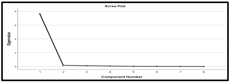
The second component percent of variance value is 2.092 and the third component percent of variance value is 1.383. But from 4th component to 8 components, all are less than 1 and the result shows that there is only one common factor. Another method to check the common factor is the scree plot method. Scree test is the graphical plotting between the eigenvalues and the eight components. A scree plot is also known as an elbow graph because the shape of the plot looks like an elbow.
| Total variance explained | ||||||
| Component | Initial eigenvalues | Extraction sums of squared loadings | ||||
| Total | % of variance | Cumulative% | Total | % of variance | Cumulative% | |
| 1 | 7.623 | 95.289 | 95.289 | 7.623 | 95.289 | 95.289 |
| 2 | 0.167 | 2.092 | 97.381 | |||
| 3 | 0.111 | 1.383 | 98.764 | |||
| 4 | 0.061 | 0.758 | 99.523 | |||
| 5 | 0.019 | 0.238 | 99.76 | |||
| 6 | 0.014 | 0.172 | 99.932 | |||
| 7 | 0.005 | 0.062 | 99.994 | |||
| 8 | 0 | 0.006 | 100 | |||
| Note: Extraction method: Principal component analysis. | ||||||
Table 7: Eigenvalues and total variance explained.
Figure 7 explains that there is only one component whose eigenvalue value is between 6 to 8 (means eigenvalue>1) and the rest of the components have less than 1 eigenvalue. So, it is clear that there all variables come under a common factor. The principal component analysis is the best extraction method to extract the large dataset into the common components. Table 8 explained that variables have a strong relationship with each other because components have greater than 0.5 loadings. Table 8 shows that variables like electric power consumption, oil consumption, coal consumption, consumption of fixed capital, household, and NPISH final consumption have extraction values nearest to 1 while the rest three variables natural gas consumption, nuclear energy consumption, and hydroelectricity consumption extraction values are lower (not near to 1). Table 9 represented the result of PCA and the orthogonal rotation method based on the Varimax method with the Kaiser normalization technique. All the components have highly loaded in one factor (F1). And the component loading values are greater than 0.9 of all the variables.
Figure 7: Scree plot between eigenvalue and number of components.
| Communalities | ||
| Initial | Extraction | |
| Electric power consumption | 1 | 0.989 |
| OIL consumption | 1 | 0.981 |
| Natural gas consumption | 1 | 0.904 |
| Coal consumption | 1 | 0.987 |
| Nuclear energy | 1 | 0.917 |
| Hydroelectricity consumption | 1 | 0.889 |
| Consumption of fixed capital | 1 | 0.978 |
| Households and NPISHs final consumption expenditure | 1 | 0.979 |
Table 8: Representation of communalities test result.
|
Component matrixa |
|
|
|
Component |
|
|
F1 |
|
Electric power consumption |
0.994 |
|
Coal consumption |
0.993 |
|
Oil consumption |
0.991 |
|
Households and NPISHs final consumption expenditure |
0.989 |
|
Consumption of fixed capital |
0.989 |
|
Nuclear energy |
0.958 |
|
Natural gas consumption |
0.951 |
|
Hydroelectricity consumption |
0.943 |
Table 9: Representation of rotated component matrix
Conclusion
In this research work, we have studied the different parameters like AIC, Normalized BIC method, RMSE, MSE, t-test, and significance level method to find out the best suitable ARIMA model for the Indian GDP growth. On the basis of this research work the ARIMA (2,3,8) is the best suitable model to forecast Indian GDP growth. And to analyze deeply the nature of variables, the factor analysis method is applied. And the research outcome is representing the interesting result that shows the high positive correlation matrix between the variables. The correlation result r>+ 0.90 between all the 8 variables. And after implementing the factor analysis it is clear that the loading of factors comes under one common factor. So, the result shows that we can reduce the size of the variables by using one (F1) common factor. The extraction representing the interesting result that shows the high positive correlation matrix between the variables. The correlation result r>+ 0.90 between all the 8 variables. And after implementing the factor analysis it is clear that the loading of factors comes under one common factor. So, the result shows that we can reduce the size of the variables by using one (F1) common factor. The extraction sums of squared loading result are 95.289% and the communality test result is explained that 7 variables (electric power consumption, oil consumption, coal consumption, natural gas consumption, nuclear energy consumption, consumption of fixed capital, and household consumption) extraction percentage is greater than 90 but only one variable (Hydroelectricity consumption) is less than 90% (88.9%).
Author Contributions
All authors have read and agreed to the published version of the manuscript.
Funding
This research received no external funding.
Data Availability Statement
Not applicable.
Conflicts of Interest
The authors declare no conflict of interest. The funders had no role in the design of the study; in the collection, analyses, or interpretation of data; in the writing of the manuscript; or in the decision to publish the results.
References
- Alina Z, Maria CD, Laura B, Georgiana-Raluca L, Corina I (2019) Factors influencing energy consumption in the context of sustainable development. Sustainability 11: 4147.
- Kentaka A, Monirul I, Arifa J (2020) Effects of COVID-19 on Indian energy consumption. Sustainability 12: 5616.
- Mona AA, Ioan P, Omer R, Mai AA, Abdulrahman SA (2021) Forecasting peak energy demand for smart buildings. J Supercomput. 77: 6356–6380.
- Junwei M (2015) The energy consumption forecasting in China Based on ARIMA model. International Conference on Materials Engineering and Information Technology Applications- Published by Atlantis Press, 192-196.
- Ohlan R (2018) Relationship between electricity consumption, trade openness, and economic growth in India. OPEC Energy Rev 42: 331-354.
- Akram J, Dina J, Amid M Mohammadreza K (2019) An autoregressive integrated moving average (ARIMA) model for the prediction of energy consumption by the household sector in the Euro area. AIMS Energy 7: 151–164.
- Sachin M, Melvin PB Abraham SP (2021) Analysis of energy consumption using RNN-LSTM and ARIMA model. J Phys 1716.
- Minglu M, Qiang W (2022) Analysis of the impact of the epidemic situation on the total electricity consumption of the United States under the prediction scenario. IOP Conf Ser: Earth Environ Sci 983.
- Guo N, Wei C, Manli W, Zijian T, Haoyue J (2021) Appling an improved method based on ARIMA model to predict the short-term electricity consumption transmitted by the Internet of Things (IoT). Wireless Communications and Mobile Computing.
- Ewa C, Joanicjusz N, Lukasz N (2021) ARIMA models in electrical load forecasting and their robustness to noise. Energies 14: 7952.
 Spanish
  Chinese
  Russian
  German
  French
  Japanese
  Portuguese
  Hindi
Hindi 