Spanish
  Chinese
  Russian
  German
  French
  Japanese
  Portuguese
  Hindi
Hindi Research Article, J Nucl Ene Sci Power Generat Technol Vol: 10 Issue: 5
The Study of Dimensional Flow of Particles and Calculation of Drag Coefficients under Different Viscosity Fluids
Rasmeet Singh*
Department of Chemical Engineering & Technology, Dr. S.S. Bhatnagar University Institute of Chemical Engineering & Technology, Panjab University, Chandigarh 160014, India
- *Corresponding Author:
- Rasmeet Singh
Department of Chemical Engineering Technology,
Dr. S.S. Bhatnagar niversity Institute of Chemical Engineering Technology,
Panab niversity,
Chandigarh 160014,
India,
Tel: 9988900108;
Email: srasmeet9@gmail.com
Received date: August, 24, 2021; Accepted date: November 18, 2021; Published date: November 29, 2021
Citation: Singh R, (2021) The Study of Dimensional Flow of Particles and Calculation of Drag Coefficients under Different Viscosity Fluids. J Nucl Ene Sci Power Generat Technol 10: 11.
Abstract
An experimental study was conducted to find the drag coefficient of small spheres of diameter 5.0, 3.45, 5.7, 5.45, and 5.20 mm under ethylene glycol, castor oil, and glycerol. Six liquids with different viscosities and densities are used so as to explore a large range of Reynolds numbers. The tubes are divided into different zones of known length. Different spherical balls of various materials and diameters are taken to observe the drag coefficient. The materials of the spherical balls are made up of glass and steel. The setup also included a stopwatch to determine the time duration of various distance intervals, a measuring scale to measure the distance of the intervals on the cylindrical tubes, a screw gauge to note down the diameters of the various spherical balls, a thermometer to note down the temperature.
Keywords: Drag coefficient, Reynolds number, Fluid flow, Stokes law.
Introduction
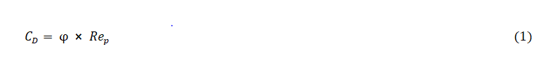
While processing fluids via pipes and channels, a friction force shows to be a useful quantity. An analogous factor known as drag coefficient is utilized for immersed solids [1, 2]. It is defined as CD = (FD/ AP)/ ρuo2/2g [3].
Where,
FD is the total drag
uo is the free stream velocity
Ap is the projected area of the particle
Dp is the diameter of the particle
For a sphere, Ap = (π/4) Dp2
For particles other than spherical, it is necessary to specify size and geometric form of the object and its orientation with respect to the direction of the flow of the fluid.
For a cylinder so oriented that its axis is perpendicular to the flow, Ap is LDp.
For a cylinder with its axis parallel to the direction of the flow, Ap is (π/4) Dp2.
From dimensional analysis, the drag coefficient of a smooth solid in an incompressible fluid depends upon a Reynolds number and necessary shape ratios. For a given shape,
The movement of a particle through a fluid requires external force acting on the particle.
Three forces act on a particle moving through a fluid:
• The external force
• The buoyant force, which acts parallel with the external force but in
opposite direction
• The drag force, which appears whenever there is relative motion
between the particle and the fluid and it acts to oppose the motion
and acts in direction opposite to that of the fluid.
Consider a particle of mass m moving through a fluid under the action of an external force Fe
U: velocity of the particle relative to the fluid
Fb: Buoyant force on the particle
FD: drag force
Then the resultant force on the particle is:
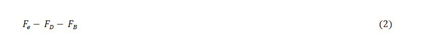
Therefore,
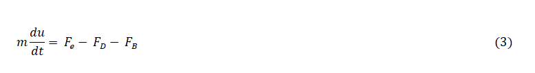
The external force can be expressed as a product of the mass and the acceleration ae of the particle from this force

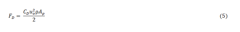
The drag force is given by
The buoyant force is, by Archimedes’ principle, the product of the mass of the fluid displaced by the particle and the acceleration from the external force and is given by
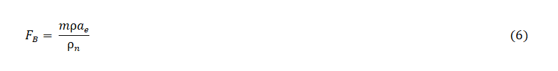
Substituting equations 4, 5, 6 in equation 3
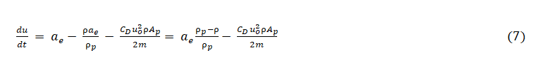
At terminal velocity put  and we get
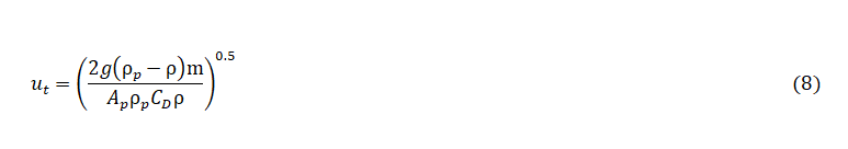
If the particles are spheres of diameter Dp
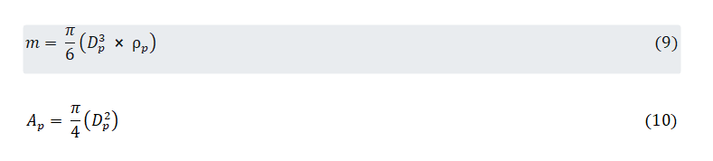
Using the above two equations in equation (7)
Stokes’ law:
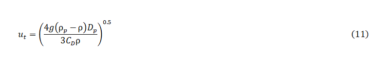
At low Reynolds numbers, the drag coefficient varies inversely with Rep and the equations for CD, FD and ut are [3, 4]:
The above equation is a form of Stokes’ law, which applies when the particle Reynolds number is less than 1.
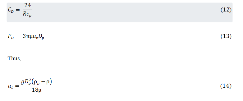
The above equation is a form of Stokes’ law, which applies when the particle Reynolds number is less than 1.
Newton’s law:
For 1000<Rep<200000, the drag coefficient is approximately constant, and the equations are
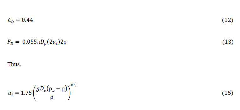
The above equation is Newton’s law and applies only for fairly large particles falling in gases or low viscous fluids.
From the equation given by Turton and Levenspiel:
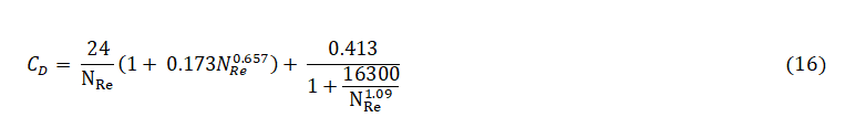
This equation defines the complete solid drag curve for < 2*
Experimental Procedure
The temperature was noted down using a thermometer.
The viscosities and densities of six different liquids taken in cylindrical tubes were noted.
5 spherical balls of different sizes and material were taken and their diameter using screw gauge was noted.
Cylindrical tube was divided into different zones of known length having a static liquid.
A spherical ball of known diameter was dropped into the cylindrical tube, taking care that it does not touch the boundaries by dropping it almost from the middle of the tube.
The time of fall of each ball in each interval was noted carefully with the help of the bulb.
For each ball the reading was taken at least three times to reduce the error.
The same procedure was repeated for the remaining tubes.
Recordings
Density of Glass = 2600 kg/m3
Density of Steel = 7800 kg/m3
| Fluid | Density (kg/m3) | Viscosity (kg/m s) |
|---|---|---|
| PIPE 1 | 900 | 0.2 |
| PIPE 2 | 911 | 0.084 |
Table 1: Properties of fluids.
| Ball | Name | Diameter (mm) |
|---|---|---|
| Big steel ball | S1 | 5 |
| Medium steel ball | S2 | 3.45 |
| Large Glass ball | G1 | 5.7 |
| Medium glass ball | G2 | 5.45 |
| Small glass ball | G3 | 5.2 |
Table 2: Specifications of balls used.
Observations
| Ball | t1 (sec) | t2 (sec) | t3 (sec) |
|---|---|---|---|
| s1 = 0.297m | s2 = 0.316m | s3 = 0.279m | |
| Small Glass Ball | 0.88 | 1.14 | 1 |
| 0.95 | 1.13 | 1.08 | |
| 1.14 | 1.17 | 1.2 | |
| Medium Steel Ball | 0.12 | 0.37 | 0.61 |
| 0.18 | 0.2 | 0.44 | |
| 0.18 | 0.45 | 0.28 | |
| 0.22 | 0.54 | 0.36 | |
| Small Steel Ball | 0.4 | 0.41 | 0.16 |
| 0.29 | 0.39 | 0.22 | |
| 0.2 | 0.41 | 0.38 | |
| 0.26 | 0.47 | 0.28 | |
| Large Glass Ball | 0.86 | 1.1 | 0.72 |
| 0.89 | 1.14 | 0.85 | |
| 0.73 | 0.84 | 0.88 | |
| 0.91 | 0.69 | 0.63 |
Table 3: Observation table for ethylene glycol.
| Ball | t1 | t2 | t3 |
|---|---|---|---|
| s1 = 0.297m | s2= 0.316m | s3= 0.279m | |
| Small Glass Ball | 20.21 | 25.49 | 22.92 |
| 21.59 | 24.21 | 22.64 | |
| 14.92 | 15.34 | 25.11 | |
| Medium Steel Ball | 4.3 | 4.52 | 4.93 |
| 4.46 | 4.99 | 6.36 | |
| 4.18 | 4.55 | 4.65 | |
| 4.2 | 4.32 | 4.59 | |
| Small Steel Ball | 6.55 | 6.58 | 6.8 |
| 6.43 | 6.63 | 6.07 | |
| 6.44 | 7.06 | 11.38 | |
| 6.43 | 6.7 | 7.26 | |
| Large Glass Ball | 17.58 | 17.81 | 19.1 |
| 17.36 | 18.8 | 20.8 | |
| 14.7 | 15.09 | 15.83 | |
| 20.71 | 22.54 | 23.68 |
Table 4: Observation table for castor oil.
| Ball | t1 | t2 | t3 |
|---|---|---|---|
| s1 = 0.297m | s2= 0.316m | s3= 0.279m | |
| Small Glass Ball | 7.23 | 6.69 | 7.49 |
| 6.78 | 7.23 | 8.45 | |
| 6.82 | 7.29 | 8.72 | |
| Medium Steel Ball | 1.38 | 1.58 | 1.48 |
| 1.41 | 1.45 | 1.69 | |
| 1.54 | 1.32 | 1.85 | |
| Small Steel Ball | 1.98 | 2.07 | 2.49 |
| 1.79 | 2.08 | 2.48 | |
| 1.83 | 2.16 | 2.46 | |
| 4.22 | 5.03 | 5.47 | |
| Large Glass Ball | 3.99 | 4.34 | 4.93 |
| 4.95 | 5.22 | 5.97 |
Table 5: Observation table for glycerol.
Calculations
| Ball | t1 | t2 | t3 | v1 | v2 | v3 | v average | Exp. Terminal Velocity | Re | Theo. Terminal Velocity | CD, experimental | CD, theoretical |
|---|---|---|---|---|---|---|---|---|---|---|---|---|
| s1 = 0.297m | s2 = 0.316m | s3 = 0.279m | ||||||||||
| Small Glass Ball | 0.88 | 1.14 | 1 | 0.3375 | 0.277193 | 0.279 | 0.297898 | 0.278602 | 6.740951 | 0.06166 | 3.5603286 | 5.7183054 |
| 0.95 | 1.13 | 1.08 | 0.3126316 | 0.279646 | 0.258333 | 0.283537 | ||||||
| 1.14 | 1.17 | 1.2 | 0.2605263 | 0.270085 | 0.2325 | 0.254371 | ||||||
| Medium Steel Ball | 0.12 | 0.37 | 0.61 | 2.475 | 0.854054 | 0.457377 | 1.262144 | 1.142446 | 31.90704 | 0.36946 | 0.7521851 | 2.0192587 |
| 0.18 | 0.2 | 0.44 | 1.65 | 1.58 | 0.634091 | 1.28803 | ||||||
| 0.18 | 0.45 | 0.28 | 1.65 | 0.702222 | 0.996429 | 1.116217 | ||||||
| 0.22 | 0.54 | 0.36 | 1.35 | 0.585185 | 0.775 | 0.903395 | ||||||
| Small Steel Ball | 0.4 | 0.41 | 0.16 | 0.7425 | 0.770732 | 1.74375 | 1.085661 | 1.013381 | 22.41776 | 0.23179 | 1.0705798 | 2.5002378 |
| 0.29 | 0.39 | 0.22 | 1.0241379 | 0.810256 | 1.268182 | 1.034192 | ||||||
| 0.2 | 0.41 | 0.38 | 1.485 | 0.770732 | 0.734211 | 0.996647 | ||||||
| 0.26 | 0.47 | 0.28 | 1.1423077 | 0.67234 | 0.996429 | 0.937026 | ||||||
| Large Glass Ball | 0.86 | 1.1 | 0.72 | 0.3453488 | 0.287273 | 0.3875 | 0.340041 | 0.357212 | 10.66791 | 0.09394 | 2.2497388 | 4.0935011 |
| 0.89 | 1.14 | 0.85 | 0.3337079 | 0.277193 | 0.328235 | 0.313045 | ||||||
| 0.73 | 0.84 | 0.88 | 0.4068493 | 0.37619 | 0.317045 | 0.366695 | ||||||
| 0.91 | 0.69 | 0.63 | 0.3263736 | 0.457971 | 0.442857 | 0.409067 |
Table 6: Calculations for ethylene glycol.
| Ball | t1 | t2 | t3 | v1 | v2 | v3 | v average | Exp. U | Re | Theo. U | CD, experimental | CD, theoretical |
|---|---|---|---|---|---|---|---|---|---|---|---|---|
| s1 = 0.297m | s2= 0.316m | s3= 0.279m | ||||||||||
| Small Glass Ball | 20.21 | 25.49 | 22.92 | 0.0146957 | 0.012397 | 0.012173 | 0.013088 | 0.0144461 | 0.083775 | 0.018866 | 286.48244 | 296.20162 |
| 21.59 | 24.21 | 22.64 | 0.0137564 | 0.013052 | 0.012323 | 0.013044 | ||||||
| 14.92 | 15.34 | 25.11 | 0.0199062 | 0.0206 | 0.011111 | 0.017206 | ||||||
| Medium Steel Ball | 4.3 | 4.52 | 4.93 | 0.0690698 | 0.069912 | 0.056592 | 0.065191 | 0.0645425 | 0.374291 | 0.104888 | 64.121256 | 69.937562 |
| 4.46 | 4.99 | 6.36 | 0.0665919 | 0.063327 | 0.043868 | 0.057929 | ||||||
| 4.18 | 4.55 | 4.65 | 0.0710526 | 0.069451 | 0.06 | 0.066834 | ||||||
| 4.2 | 4.32 | 4.59 | 0.0707143 | 0.073148 | 0.060784 | 0.068216 | ||||||
| Small Steel Ball | 6.55 | 6.58 | 6.8 | 0.0453435 | 0.048024 | 0.041029 | 0.044799 | 0.0434492 | 0.251968 | 0.065805 | 95.250217 | 101.91209 |
| 6.43 | 6.63 | 6.07 | 0.0461897 | 0.047662 | 0.045964 | 0.046605 | ||||||
| 6.44 | 7.06 | 11.38 | 0.046118 | 0.044759 | 0.024517 | 0.038465 | ||||||
| 6.43 | 6.7 | 7.26 | 0.0461897 | 0.047164 | 0.03843 | 0.043928 | ||||||
| Large Glass Ball | 17.58 | 17.81 | 19.1 | 0.0168942 | 0.017743 | 0.014607 | 0.016415 | 0.0162906 | 0.094471 | 0.028742 | 254.04528 | 263.37201 |
| 17.36 | 18.8 | 20.8 | 0.0171083 | 0.016809 | 0.013413 | 0.015777 | ||||||
| 14.7 | 15.09 | 15.83 | 0.0202041 | 0.020941 | 0.017625 | 0.01959 | ||||||
| 20.71 | 22.54 | 23.68 | 0.0143409 | 0.01402 | 0.011782 | 0.013381 |
Table 7: Calculations for castor oil.
Calculations for glycerol.
| Ball | t1 | t2 | t3 | v1 | v2 | v3 | v average | Exp. U | Re | Theo. U | CD, experimental | CD, theoretical |
|---|---|---|---|---|---|---|---|---|---|---|---|---|
| s1 = 0.297m | s2= 0.316m | s3= 0.279m | ||||||||||
| Small Glass Ball | 7.23 | 6.69 | 7.49 | 0.041079 | 0.047235 | 0.03725 | 0.041854 | 0.040554 | 0.126759 | 0.006331 | 189.33532 | 197.76742 |
| 6.78 | 7.23 | 8.45 | 0.043805 | 0.043707 | 0.033018 | 0.040177 | ||||||
| 6.82 | 7.29 | 8.72 | 0.043548 | 0.043347 | 0.031995 | 0.03963 | ||||||
| Medium Steel Ball | 1.38 | 1.58 | 1.48 | 0.215217 | 0.2 | 0.188514 | 0.201244 | 0.197828 | 0.618352 | 0.041194 | 38.812831 | 43.709094 |
| 1.41 | 1.45 | 1.69 | 0.210638 | 0.217931 | 0.165089 | 0.197886 | ||||||
| 1.54 | 1.32 | 1.85 | 0.192857 | 0.239394 | 0.150811 | 0.194354 | ||||||
| Small Steel Ball | 1.98 | 2.07 | 2.49 | 0.15 | 0.152657 | 0.112048 | 0.138235 | 0.140784 | 0.44005 | 0.041194 | 54.53929 | 60.041499 |
| 1.79 | 2.08 | 2.48 | 0.165922 | 0.151923 | 0.1125 | 0.143448 | ||||||
| 1.83 | 2.16 | 2.46 | 0.162295 | 0.146296 | 0.113415 | 0.140669 | ||||||
| 4.22 | 5.03 | 5.47 | 0.070379 | 0.062823 | 0.051005 | 0.061403 | 0.061702 | 0.192862 | 0.009645 | 124.4412 | 131.7428 | |
| Large Glass Ball | 3.99 | 4.34 | 4.93 | 0.074436 | 0.072811 | 0.056592 | 0.067946 | |||||
| 4.95 | 5.22 | 5.97 | 0.06 | 0.060536 | 0.046734 | 0.055757 | ||||||
Results

Figure 1: Plot of CD experimental versus CD theoretical.

Figure 2: Plot of CD experimental versus Reynolds number.

Figure 3: Plot of U theoretical versus U experimental.

Figure 4: Plot of CD experimental versus CD theoretical.

Figure 5: Plot of CD experimental versus Reynolds number.

Figure 6: Plot of U theoretical versus U experimental.

Figure 7: Plot of CD experimental versus CD theoretical.

Figure 8: Plot of CD experimental versus Reynolds number.

Figure 9: Plot of U theoretical versus U experimental.
Discussion of Result
From the experiment we studied the nature of different fluids of different densities and viscosities. We saw the variation in drag coefficient by varying the Reynolds No. i.e. we used spherical balls of various materials as well as diameters. We saw there were quite discrepancies in the experimental and the theoretical plot of velocity and coefficient of drag vs Reynolds no. The discrepancies may be due to parallax, error in noting the time, wall effects, instrumental error due to screw gauge in measuring the diameter and human error might also have crept in due a large no. of people working at the same time.
References
- Selberg BP, JA Nicholls (1968) "Drag coefficient of small spherical particles." AIAA Journal 6, no. 3: 401-408.
- Alam F, Steiner T, Chowdhury H, Moria H, Khan I, Aldawi F. and Subic A (2011) A study of golf ball aerodynamic drag. Procedia Engineering, 13, pp.226-231.
- McCabe, WL, Smith, JC. and Harriott, P (1993) Unit operations of chemical engineering 5, p.154. New York: McGraw-hill.
- Sutterby JL (1973) Falling sphere viscometry. I. Wall and inertial corrections to Stokes' law in long tubes. Transactions of the Society of Rheology, 17(4), pp.559-573.