Spanish
  Chinese
  Russian
  German
  French
  Japanese
  Portuguese
  Hindi
Hindi Research Article, Res Rep Math Vol: 2 Issue: 1
A Multiply Nested Model for Non-Linear Shallow Water Model
Huda Altaie*
Laboratoire JA Dieudonne (mathematiques) UMR CNRS 7351, Universite de Nice -Sophia Antipolis, France
*Corresponding Author : Huda Altaie
Laboratoire JA Dieudonne (mathematiques) UMR CNRS 7351, Universite de Nice -Sophia Antipolis, France
Tel: +33 4 92 07 69 96
E-mail: Huda.AL_TAIE@unice.fr
Received: August 17, 2017 Accepted: January 29, 2018 Published: February 05, 2018
Citation: Altaie H (2018) A Multiply Nested Model for Non-Linear Shallow Water Model. Res Rep Math 2:1
Abstract
The principle objective of this paper is to study the accuracy and efficiency of two-way performance nesting techniques for structured grids between a coarse grid and a fine grid for 2D shallow water models using explicit finite difference scheme. This model consists of a higher- resolution (fine grid) model with nested 3:1 embedded in a low-resolution (coarse grid) model on which covers the entire domain. The formulation of the mesh nesting algorithm of the structure grid model allows flexibility in deciding the number of meshes and the ratio of grid resolution between adjacent meshes. The two- way nesting is satisfied with an interpolating of the coarse grid domain to provide boundary conditions for the fine grid region and by updating the variables on the fine grid is suit- ably averaged onto the coarse grid in order to drive the coarse grid model. Comparing the results of a fine grid and a coarse grid shows the two- way nesting technique to be working efficiently over different periods of time and these results indicate good performance of the nesting technique.
Keywords: Shallow water equations; Numerical models; Multi-nested; Adaptive scheme
Introduction
Nesting is a fine mesh within a coarse mesh grid model represents an economical way to improve the horizontal resolution in ocean models and weather models. Best resolution of the horizontal scale can be obtained without requiring a fine resolution grid throughout the full model domain. This allows a more accurate solution to the Ocean thus, saving computer time and memory space.
A large number of researchers have used such multiply nested grids primarily to provide a more gradual change between grid meshes and to give smoother solutions near the boundary. The nested method involves the embedding of a higher resolution grid into a lower resolution grid, which covers the full model do- main. There are two main types of nesting procedures, a one-way or passive method a two-way or interactive nesting method [1-4].
Admonitions to use two-way nesting have occasionally seen in the literature [5,6], but the few examples given supporting this assertion do not show a dramatic difference between one-way and two-way nesting and one-way nesting is still used in some applications.
Sundstrom and Elvius [6] claim that two-way nesting may give larger errors than one-way nesting because of reactions caused by the change of phase speeds between the nested and coarse grids; however, they also do not give any examples supporting this assertion and further- more do not consider similar effects when using one-way nesting.
Phillips and Shukla [2] compared the re- actions of nonlinear two-dimensional shallow- water Rossby and gravity waves off of the inter- face of both one-way and two-way nested grids. They found that the solutions for a two-way nest were (almost invariably nearer) to a single- grid control case with the same resolution as the nested grid; however, they did not give any rigorous explanation for this beyond the basic fact that the coarse grid solution is influenced by that of the nested grid over the region on which the two grids coincide.
Clark and Farley [5] performed a one-way simulation of vertically propagating mountain waves that was considerably noisier than the same simulation performed with a two-way nest, but the majority of the errors in their one-way nest appeared to be due to reactions off of the nested grids upper boundary, which did not coincide with the coarse grids upper boundary.
Rothstein and Ginis [7] and Shukla J Phillips [2] constructed a numerical technique to develop a two-way movable nested grid for meteorological applications. The grid points were not staggered and all meteorological variables have been defined at the same point.
Based on the literature reviewed, a two-way nesting technique can be used to embed a high- resolution grid into a lower-resolution grid of the entire domain, with interaction between the two domains occurring. Interaction between the two domains occurs by a coarse (parent) grid providing boundary conditions for the nested (child) domain and the high-resolution nested (child) grid solution is used to update a coarse (parent) grid solution in a common area. Through this approach the computational cost of a hydrodynamic model can be reduced. Two-way nesting techniques enable local characteristics in an area of interest to be modelled with a high level of accuracy, as well as showing how these features propagate into and affect the surrounding do- main in the low resolution area [8,9].
The present paper is arranged as follows: Description the nesting model in section
In section 3, discuss some numerical examples of 2D non-linear shallow-water model using explicit center finite difference and leapfrog schemes with Asselin-Roberts filter and compare the results when the model has the spacial refinement ratio 1: 3. Finally, in section 4, the main conclusions are summarized.
Description of Model
Governing equations
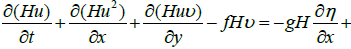
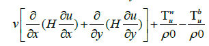
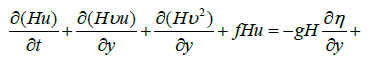
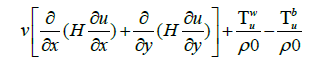
Consider the 2D depth-averaged nonlinear shallow water equation which contains the as follows (see [10,11]):
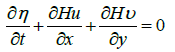
Where
x, y are the horizontal coordinates
t is the time
u=u (x,y,t) is the depth-averaged horizontal velocity in the x direction
v=v (x,y,t) is the depth-averaged horizontal velocity in the y direction
H=H (x,y,t) is the depth from the surface level to the bottom(water height)
ν is the horizontal turbulent viscosity
g stains for the gravity acceleration
f = 1.01 × 10⁻⁴ rad/s is the Coriolis fre- quency at 42° of latitude
ρ0 = 1033 kg/m3 is the water mean density.
η is the water level relative to rest
 is the bottom stress zonal component and
 is the wind stress zonal component
The finite difference scheme used in this model is based upon the alternating explicit center finite difference scheme in space and explicit leapfrog scheme with Asselin-Roberts filter in time by using t open boundary condition, we use linear interpolated scheme at end of time step in coarse grid domain and updating by averaging method at each end of time step in fine grid domain.
One-way nested methods
One-way nesting is applied on the models to generate a higher level of resolution in an area of interest. The nested domain is positioned so it is embedding the coarse domain. There are two kinds of the schemes for the running of a one- way nesting technique. The first scheme involves on the complete separation of the coarse and fine models with respect to simulation time. In this method, the coarse model is fully run for the model simulation time. The data required for the boundary conditions are stored in a data file to be used for the fine domain model that is then fully run for the simulation time. This method is known as an uncoupled modeling procedure.
The coupled modeling procedure is more at- tractive than the uncoupled, as it does not require large amounts of storage. In this method, the coarse model is run for one-time step and data required for the nested domains boundary conditions are assigned allowing the fine model to proceeds to a time step equal to the coarse domains. The coarse domain only proceeds to the next time step when the fine domain has been integrated [12,13].
Two-way nested methods
In a two-way nested model the coarse and fine grids are by necessity dynamically linked each influences the other and neither can be run in- dependently. The interaction in the direction of coarse to fine is similar in manner to one-way nested systems. The coarse model is integrated in time and the boundary conditions of the fine model are interpolated (in time and space) from adjacent parent grid points the fine model is the nested domain was contained entirely in a low - resolution coarse domain. Interaction between the two domains occurred through the interpolation of the coarse grid data at the interface between the two domains to provide boundary conditions for the nested domain, the high- resolution nested domain solution was used to update the coarse solution in the zone where the two domains overlap. The interaction between the two domains occurring in an area called the dynamic interface located near the nested domain boundary [8,13].
The following figure shows an illustration of the grid configuration for a nested ratio of 3:1 (Figure 1).

Figure 1: Illustration of the grid configuration for a nested ratio of 3:1.
Two-way nesting algorithm (nesting procedure)
The information on values fluxes and free- surface is exchanged on the boundaries between two nested grid regions. At each new time level, the values fluxes on the boundary of a finer grid are obtained by linearly interpolating both spatially and temporally, the values fluxes obtained from its outer parent grid. At each next time level for the outer parent grid, the free-surface on a coarser grid is updated by averaging, both spatially and temporally the free surface obtained on the inner finer grid. The procedure described holds for every pair of coarse and fine grid it can be summarised as follows:
Suppose all flux values in the finer and the coarser region are known at time level t = nΔt and we need to solve the finer region and the coarser region values at the next time step t = (n + 1)Δt. Since the coarser grid region and the finer grid region adopt different grid sizes, the time step sizes for each region are different due to the requirement of stability.
Case1: The time step of the finer region is one half of the coarser region
(a)-For the coarse model (outer domain):
i) Solve continuity equation to find  using horizontal / velocity components
  and
and  at time level n. Elevations at time level (n−1/2) and the total depth H at time level (n-1/2)
ii) Solve momentum equations for and  using
using  .
.
(b)-For the fine model (inner domain):
The algorithm for the fine model requires more steps than the coarse model depending on the temporal refinement factor The following illustrates the situation where the temporal refinement factor p=2.
1. Solve continuity equation for  using
using  and certain values of
  and
and  which coincide with the fine grid open boundary points.
2. Solve momentum equations for and  using
using 
3. Transform  and
and  from coarse grid onto fine grid and update model time
4. Solve continuity equation for  using
using 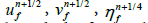 certain values of
  and
and  which coincide with the fine grid open boundary points.
5. Transform  from fine grid onto coarse grid using linear interpolation and update model time.
6. Solve momentum equations for  and
and  using
using 
Case2: The space and time refinement factor is 1:3
Step 1. Get the free surface elevation at t = (n + 1)Δt
Step 2. Get the free surface elevation at t = (n + 1/3)Δt in the inner region by solving continuity equation.
Step 3. Get the flux values at t = (n+2/3)Δt in the inner grid region by solving momentum equation.
Step 4. Get the free surface elevation at t = (n + 1) Δt in the inner grid region by solving continuity equation, in this case the information of free surface transfer from inner to outeg by copy grids using dirchelet conditions.
Step 5. Get the flux values at t = (n + 4/3) Δt in the inner grid region by solving momentum equation.
Step 6. Get the free surface elevation at t = (n + 5/3) Δt in the inner grid region by solving continuity equation.
Step 7. Get the flux values at t = (n+2) Δt in the inner region by solving momentum equation.
Step 8. Get the flux values at t = (n+2) Δt in the outer region by solving momentum equation using free surface elevation at t = (n + 1) Δt (updated)
Feedback of Boundary Data
Interpolation techniques are required for effective data transmission as data is transferred between domains of different spatial and temporal resolution. There are two main goals for an interpolation scheme to be optimum: (1) to maximize the information being transferred and (2) to minimize the generation of noise.
Interpolation techniques used in the transfer of information from the coarse domain to the nested domain are usually of a polynomial form or a linear/bilinear form.
Problems can arise with the use of polynomial techniques in areas of sharp gradients due to the formation of surplus oscillation of the interpolation variables. Therefore linear interpolation is more widely used for both spatial and temporal interpolation.
There are four main updating interpolation procedures for the transfer of information from the fine domain into the coarse domain (1) direct copy (2) basic averaging procedure (3) Shapiro and (4) fully weighted averaging procedure [1].
(1)- Direct copy is the most severe interpolation technique with only the nested grid point that lies directly in the region of the coarse grid point being used in the procedure.

where  represents the coarse grid point and
 represents the nested grid point that over-lays the centre of the coarse grid cell.
(2)- The average procedure takes into account all fine grid points that are enclosed in the coarse cell [2]. This scheme is based on the assumption that the _ne grid variables over laying the one coarse grid cell have a uniform distribution of value.

 representing the coarse point that is being updated and ,
 being the fine grid values in the same cell.
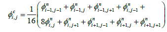
(3)-The Shapiro interpolation scheme is based on the assumption that the nested grid point that lies in the central region of the coarse grid is of equal importance to the sum of the other nested grid points enclosed in the coarse grid cell [1].
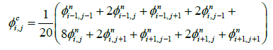
(4)- The _nal interpolation scheme is the full weighted averaging method and assumes that the interpolated value used for the updating procedure should be influenced mainly by nested grid points close to the centre of the coarse grid point being updated and less by the more distant points [9].
Spatial and Temporal Refinements
The grid element, the basic unit of the grid consists of three grid points which are the free surface elevation and the horizontal velocity components u and u with the spatial refinement factor being an odd integer m which is defined by:

where Δλc and Δλf are the coarse and fine grid lengths respectively.
In the present model the refinement factor are 1:3 so the scheme is called a one-third-refinement model if the refinement factor is 3.
In this model refinement in time as well as space is carried out so the coarse spatial model uses the large time steps and the fine spatial model the small time steps.
The general finite difference scheme used for both grids is threelevel in time .The time levels in one time step of the coarse grid and the corresponding levels in two equivalent time steps of the fine grid. It should be noted that the temporal refinement factor is defined by the integer ρ given by 
Results
This section highlights for a new technique of two-way nesting and Discuss some numerical examples of the 2D non-linear shallowwater model using explicit center finite difference and leapfrog schemes with Asselin-Roberts filter with Dirichlet open boundary condition, we use interpolated scheme at the end of time step in the fine grid domain and updating by averaging method at each end of time step in the coarse grid domain. Also, Compare the results when the model has the spatial refinement ratio 1: 3. Finally, Coupling systems for the 2D non-linear shallow water equations are applied.
Example 1
In this example, we find the absolute error and relative error l2 in one-way and two way nesting for 2D depth averaged nonlinear shallow water equations with non-rotated f=0 , _ = 0, wind and bottom stress =0, the space and temporal refinement ratio is 1:3 at different value of time t= 10,20,30,40,50,100,200 days, when nx=ny=120 , dx=dy=9 , dt=0.01 in coarse grid, nx=ny=120 , dx=dy=3, dt=0.003 in fine grid using Dirichlet open boundary condition, the interpolation techniques used in the transfer of information from the coarse domain to the nested
domain are usually of a polynomial form or a linear form and for updating interpolation used average procedures.
The following figures represent the relative error l2 in one-way and two- way nesting grids (Figure 2).

Figure 2: Relative error l2 in one-way and two- way nesting grids.
Case 1: When the space refinement ratio is 1:3 and the temporal refinement ratio is 1:2
Example 2
In this example, we use a system of 2D depth-averaged linear shallow water equations (wind stress=0, non-rotated f=0) for finding the relative error l2 of the free surface in two-way nesting grid when the coarse grids contain more than one finer grid at difference times t=500 ,1000,... 4000 hour, nx=ny=120,dx=dy=9,time step=0.025 in coarse grid (the information about the coarse and fine grids are given in Table 1.)
| Information | Grid 01 | Grid 21 | Grid 22 | Grid 31 | Grid 32 |
|---|---|---|---|---|---|
| No. of grids | 120×120 | 120×120 | 120×120 | 120×120 | 120×120 |
| length grid size | 9 | 3 | 3 | 1 | |
| parent grid | non | grid 01 | grid 01 | grid 21 | grid 22 |
| grid size ratio | non | 3 | 3 | 3 | 3 |
| time step in sec | 0.025 | 0.013 | 0.013 | 0.0063 | 0.0063 |
| SWEs | non-linear | non-linear | non-linear | non-linear | non-linear |
| Latitude | 31-70 | 61-100 | Jan-40 | 41-80 | |
| longitude | Nov-50 | 61-100 | Nov-50 | 41-80 | |
| CFL | — | 0.7 | 0.7 | 0.6 | 0.6 |
Table 1: Shows the information for the different grids for the 2D non- linear shallow water model.
The following figure shows the comparison for relative error l2 between (coarse grid in level 1 and grid 21 in level 2) and relative error l2 between (coarse grid in level 1 and grid 22 in level 2) at different times of t=500,1000,...,4000 (hours) (Figure 3).

Figure 3: Comparison for relative error l2 between (coarse grid in level 1 and grid 21 in level 2 ) and relative error l2 between (coarse grid in level 1 and grid 22 in level 2) at different times of t=500,1000,...,4000 (hours) .
Example 3
In this example, we use a system of 2D depth- averaged linear shallow water equations (wind stress=0, non-rotated f=0 ) for finding the relative error l2 when a fine grids contain again one finer grid in another level (multi level) at difference times t=500 ,1000,... 4000 hour, when nx=ny=120,dx=dy=9, time step=0.025 in coarse grid (the information about the coarse and fine grids are given in Table 1).
The following figure shows the comparsion for the relative error l2 in (level 1- level 2) and (level 2-level 3) at different times of t=500, 1000,...,4000 (hours) (Figure 4).

Figure 4: Comparsion for the relative error l2 in (level 1- level 2) and (level 2-level 3) at different times of t=500,1000,...,4000 (hours).
Example 4
In this example, we find the relative error l2 for the 2D depth averaged nonlinear shallow water equation (V=0, the wind stress =0, f=0) when the coarse grids contain more than one finer grid at difference times t=500, 1000,...4000 hour, when nx=ny=120, dx=dy=9, time step=0.025 in the coarse grid (the information about the coarse and fine grids are given in Table 1)
The following figure shows the comparison for the relative error l2 between (coarse grid in level 1 and grid 21 in level 2) and the relative error l2 between (coarse grid in level 1 and grid 22 in level 2) at different times of t=500,1000,...,4000 (hours) (Figure 5).

Figure 5: Comparison for the relative error l2 between (coarse grid in level 1 and grid 21 in level 2) and the relative error l2 between (coarse grid in level 1 and grid 22 in level 2) at different times of t=500,1000,...,4000 (hours).
Example 5
In this example, we find the relative error l2 for 2D depth averaged nonlinear shallow water equation (v=0, the wind stress =0, f=0) when _ne grids contain again one finer grid in another level at difference times t=500, 1000,...4000 hour, when nx=ny=120, dx=dy=9, time step=0.025 in the coarse grid(the information about the coarse and fine grids are given in Table 1).
The following figure compares the relative error l2 between level 2 (grid 21) and level 3 (grid 31) at different times of t=500, 1000,..., 4000 (hours).
Example 6
In this example, we find the relative errorl2 for 2D depth averaged nonlinear shallow water equation (v=0, the wind stress =0, f=0) when the second _ne grid contains again one finer grid in another level at difference times t=500, 1000,...4000 hour, when nx=ny=120,dx=dy=9, time step=0.025 in the coarse grid(the information about the coarse and fine grids are given in Table 1)
The following figure compares the relative error l2 between (fine grid 22 in level 2 and fine grid 32 in level 3) and (fine grid 21 in level 2 and fine grid 31 in level 3) at different times of; t=500,1000,...,4000 (hours) (Figure 6).

Figure 6: Comparision for the relative error l2 between level 2 (grid 21) and level 3 (grid 31) at different times of t=500,1000,...,4000 (hours).
Example 7
(Case 1: Coupling (embedding) systems for 2D nonlinear shallow water equations.)
In this example, we find the relative error l2 for 2D depth averaged nonlinear shallow water equation (v, wind stress and f=0), when the coarse grids contain only one finer grid at difference times t=500, 1000,... 4000 hr, when nx=ny=120, dx=dy=9, time step=0.020 in the coarse grid (the information about the coarse and fine grids are given in Table 1)
The following figure Compares of the relative error l2 between level 1, level 2 and level 2,level 3 in case nonlinear shallow water equations (Figure 7).

Figure 7: Comparision for the relative error l2 between (fine grid 22 in level 2 and fine grid 32 in level 3) and (fine grid 21 in level 2 and fine grid 31 in level 3 ) at different times of t=500,1000,...,4000 (hours).
Example 8
Case 2: Coupling systems for 2D linear / nonlinear shallow water equations.
In this example, we find the relative error l2 for 2D depth averaged nonlinear shallow water equation (v= 0, the wind stress =0, f=0) when the coarse grids contain more than one finer grid at difference times t=500, 1000,... 4000 hour, when nx=ny=120, dx=dy=9, time step=0.020 in the coarse grid (the information about the coarse and fine grids are given in Table 1.)
In this case, By solving the system of 2D depth averaged nonlinear shallow water equations in 1st-level which contains a coarse grid and coupling (embedding) with the system of 2D depth averaged nonlinear shallow water equations in 2nd-level which contains a fine grid also, coupling (embedding) this system with the system of 2D depth averaged linear shallow water equations in the 3rd-level which contain another finer grid.
The following figure Compares for the relative error l2 between level 1, level 2 and level 2,level 3 using Dirichlet open boundary condition, we use interpolated scheme at end of time step in coarse grid domain and updating by averaging method at each end of time step in fine grid domain. It Compares of the relative error l2 between (level 1, level 2) in case non-linear and (level 2, level 3) in case nonlinear to linear 2d depth averaged shallow water equation (Figure 8).

Figure 8: Comparision of the relative error l2 between level 1, level 2 and level 2,level 3 in case nonlinear shallow water equations.
Example 9
Case 3: Coupling systems for 2D nonlinear / linear shallow water equations
In this example, we find the relative error l2 for 2D depth averaged nonlinear shallow water equation (v= 0, the wind stress =0, f=0) at difference times t=500, 1000,...4000 hr, when nx=ny=120,dx=dy=9, time step=0.020 in coarse grid(the information about the coarse and fine grids are given in Table 1).
In this case, when solving the system of 2D depth averaged nonlinear shallow water equations in 1st-level which contains a coarse grid and coupling (embedding) with the system of 2D depth averaged linear shallow water equations in 2nd-level which contains a finer grid also, by coupling (embedding) this system with the system of 2D depth averaged nonlinear shallow water equations in the 3rdlevel which contain another finer grid .The following figure Compares for the relative error l2 between level 1,2 and level 2,3using open boundary condition, we use interpolated scheme at end of time step in coarse grid domain and updating by averaging method at each end of time step in fine grid domain.
The following figure Compares of the relative error between levels 1, level 2 in case nonlinear to linear and level 2, level 3 in case linear to nonlinear 2d shallow water equation (Figures 9 and 10).

Figure 9: Comparision of the relative error l2 between (level 1, level 2) in case non-linear and (level 2,level 3) in case nonlinear to linear 2d depth averaged shallow water equation.

Figure 10: Compares of the relative error between level 1, level 2 in case nonlinear to linear and level 2, level 3 in case linear to nonlinear 2d shallow water equation.
Summary and Conclusion
Accuracy and efficiency are two main indicators in evaluating the performance of the numerical models. The approach introduced in the paper presented the possibility of increasing accuracy and efficiency of the modelling results within a two-way nesting grid model. A new technique of two-way nesting algorithm is proposed. To verify the nested multiply grid model, several numerical examples were presented and it was shown that two way nesting techniques perform better than the one-way nesting technique. In particular, two-way nesting ensures dynamical consistency between a coarse grid and a fine grid occurs frequently. Also, when using the ratio grid size 1:3 the connecting boundary conditions is very well. In general, good results are observed.
References
- Zhang DL, Chang HR, Seaman NL, Warner TT, Fritsch JM (1986) A two-way interactive nesting procedure with variable terrain resolution. Mon Weather Rev 114: 1330-1339.
- Phillips NA, Shukla J (1973) On the strategy of combining coarse and Fine grids meshes in numerical weather prediction J Appl Meteorol 12: 763-770.
- Kurihara Y, Tripoli GJ, Bender MA (1979) Design of a movable nested-mesh primitive equation model. Mon Weather Rev 107: 239-249.
- Harrison Jr EJ (1973) Three-dimensional numerical simulations of tropical systems utilizing nested finite grids. J Atmospheric Sci 30: 1528-1543.
- Clark TL, Farley RD (1984) Severe downslope windstorm calculations in two and three spatial dimensions using anelastic interactive grid nesting: A possible mechanism for gustiness. J Atmospheric Sci 41: 329-350.
- Sundström A, Elvius T (1979) Computational problems related to limited area modelling. Numerical methods used in atmospheric models 2: 379-416.
- Ginis I, Richardson RA, Rothstein LM (1998) Design of a multiply nested primitive equation ocean model. Mon weather Rev 126: 1054-1079.
- Debreu L, Marchesiello P, Penven P (2009) Two-Way embedding algorithms for a split-explicit free surface ocean model. Ocean Modell., In preparation.
- Kantha LH, Clayson CA (2000) Numerical models of oceans and oceanic processes. Academic press, USA.
- Garcıa-Navarro P, Brufau P, Burguete J, Murillo J (2008) The shallow water equations: An example of hyperbolic system. Monografıas de la Real Academia de Ciencias de Zaragoza 31: 89-119.
- Spall MA, Robinson AR (1989) A new hybrid coordinate open ocean primitive equation model. Math Comput Simul 31: 241-269.
- Pullen J, Allen JS (2001) Modeling studies of the coastal circulation off northern California: statistics and patterns of wintertime flow. J Geophys Res 106: 26959-26984.
- Oey LY, Chen P (1992) A nestedâ€Âgrid ocean model: With application to the simulation of meanders and eddies in the Norwegian Coastal Current. J Geophys Res 97: 20063-20086.