Research Article, Geoinfor Geostat An Overview Vol: 0 Issue: 0

Comparative Analysis of Spatial Interpolation Techniques for Rainfall Over Hassan District, Karnataka, India

Shambhavi Aravind Kaushik¹, Madhu Kumar K¹, Vinay M², Pushpa Tuppad^3*

¹Department of Environmental Engineering, Sri Jayachamarajendra College of Engineering, Mysuru, Karnataka, India

²Department of Studies in Geography, Manasagangothri, University of Mysore, Mysuru, Karnataka, India

³Department of Environmental Engineering, JSS Science and Technology University, Sri Jayachamarajendra College of Engineering, Mysuru, Karnataka, India

Corresponding Author: Pushpa Tuppad
Department of Environmental Engineering, JSS Science and Technology University, Sri Jayachamarajendra College of Engineering, Mysuru, Karnataka, India
E-mail: ptuppad@sjce.ac.in

Received: August 22, 2021 Accepted: September 06, 2021 Published: September 13, 2021

Citation: Kaushik SA, Madhu Kumar K, Vinay M, Tuppad P (2021)  Comparative Analysis of Spatial Interpolation Techniques for Rainfall Over Hassan District, Karnataka, India. Geoinfor Geostat: An Overview 9:9.

Abstract

Keywords: Interpolation, IDW, Kriging, Trend, Spline, Python, Exceedance probability

Introduction

Measured rainfall data using rain gauges, although point information, is highly valuable. To effectively capture spatial variability of rainfall over a region requires setting up of a number of such measuring instruments, which necessitates huge installation and operational costs, especially when the area concerned is large. In order to overcome this problem, GIS and geostatistical interpolation techniques are very promising. The rainfall data of different time scales for the area of interest of a given period, from a finite number of stations, can be subjected to interpolation to obtain spatial information [1]. The spatially interpolated dataset can then be developed into aerial telemetry maps. This technique could provide accurate and reliable estimates of data at locations where no measurements are available. The precipitation data finds itself of vital use in prediction and modelling of floods, droughts, cyclones, climate studies [2,3], agricultural and natural resources management [4], and soil moisture studies [5] , rainfall-runoff estimation [6] and so on.

As rainfall is a highly variable parameter, both in space and time, reliable spatial interpolation of rainfall is inherently more difficult to carry out compared to the interpolation of other parameters [7]. Coarse spatial and temporal resolution of measured rainfall makes the utility of interpolation techniques limited [4]. It is important to note that the performances of the interpolation techniques are usually region-specific. This means that different techniques have different accuracies for different places, depending on meteorological, topographical and environmental conditions. Therefore, it is crucial to select the best interpolation technique for a given area to obtain reasonably accurate results. Inverse Distance Weighting (IDW) method, Kriging, nearest neighbour, Spline, and trend are some of the methods used to interpolate the attribute data to unsampled locations. IDW technique implements the assumption that the value of an attribute at an unknown location is inversely related to the distance of a known point from it. Thus, points closer to an estimating location will have a higher weight (as a function of the distance between the two points) assigned to it, as compared to a point that is farther away from the estimating point [8]. Kriging technique uses a variogram to characterise the spatial correlation and produce a combination of measured values, based on the type of variogram [9,10]. Nearest neighbour interpolation assigns the measured values of the nearest rain gauge to the estimating point [11]. Spline is a type of deterministic method that uses a polynomial to fit the measured values and produce a smoothly varying surface. The estimating value by spline is obtained from a specific point, defined by a radius and these points are adapted to the values at the measured location [12]. Trend surface interpolation uses a linear equation to fit the measured values into a smooth surface.

Numerous experiments have been conducted to interpolate the rainfall averages over different time scales, in different regions [13]. Compared the spatial interpolation techniques (kriging with its variants, IDW, spline, trend and natural neighbour) for their accuracy in interpolating 30-year mean annual rainfall for the Mysuru and Chamarajanagar Districts in Karnataka, India. They reported that, for the regions with similar characteristics to that of their study area, ordinary kriging works best, followed by IDW and universal kriging. Another study conducted in Tunisia to interpolate the annual rainfall, reported that ordinary kriging yields RMSE of 3.443 and Mean error (ME) of 0.038 for 75 samples [14,15]. Mapped annual precipitation in the middle Ebro Valley (Spain) and concluded that regression based models performed better than the local interpolators, especially when they use four geographic and topographic variables. Among the deterministic methods, spline gave low RMSE values making it more suitable for the study area compared to IDW and trend interpolation. Scientific literature suggests that the spatial interpolation techniques perform better when the precipitation data is supplemented with auxiliary variables such as elevation and temperature [16] investigated the performance of simple kriging with varying local means, kriging with an external drift, and co-located cokriging, when a digital elevation model is incorporated into the estimation. They found that kriging with varying local means performed best for interpolation of monthly rainfall data and kriging with external drift gave slightly better results than the more complex cokriging for interpolating annual rainfall. However, it is not always true that use of elevation data will enhance the performance of geostatistical techniques to interpolate rainfall. Comparison of ordinary kriging, ordinary cokriging and kriging with external drift to produce monthly and annual rainfall maps for the Hawaiian Islands showed that ordinary kriging outperformed the other techniques, considering the months from January 1920 to December 2012 [17]. Their overall cross- validation results indicated that for the sample months considered, ordinary kriging did not significantly differ from the techniques that incorporated a secondary “elevation” variable.

All interpolation models have a fundamental requirement that the dataset is complete on a spatial  and temporal basis. Spatial interpolation techniques developed for specific data types or variables can be applied to various disciplines like environmental sciences, hydrology, mining engineering, meteorology, etc. With change in atmospheric conditions, the time scale chosen to evaluate the interpolation techniques becomes crucial, as the validity of an interpolation technique changes annually, monthly, seasonally and also on a daily basis.

The objectives of this study were to perform spatial interpolation on continuous time series of precipitation data using IDW, Trend, Spline and Kriging, and cross-validate to assess the accuracy of these techniques at different temporal scales.

Study Area

The study area chosen is the Hassan District in Karnataka, India Figure 1. It is one of the 30 Districts located in the south-western part of Karnataka, lying between 12013 and 13033 north latitudes and 75033 and 76038 east longitude. It has a total area of 6826.15 km2, with the greatest length of about 129 km extending from south to north and greatest width of about 116 km from east to west. The District has 8 taluks: Hassan, Alur, Arkalgud, Arsikere, Belur, Channarayapatna, Holenarasipura and Sakaleshpura Figure 1, 38 hoblies and 2369 villages. Annual average rainfall in the study area is about 1031mm and the major agricultural crops grown are coffee, paddy, sugarcane, black pepper and potato. Hassan District lies partly in the “Malnad” (hilly land) tract and partly in the southern “Maidan” (plains) tract.

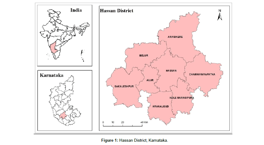
Figure 1: Hassan District, Karnataka.

The study area chosen is the Hassan District in Karnataka, India Figure 1. It is one of the 30 Districts located in the south-western part of Karnataka, lying between 12013 and 13033 north latitudes and 75033 and 76038 east longitude. It has a total area of 6826.15 km2, with the greatest length of about 129 km extending from south to north and greatest width of about 116 km from east to west. The District has 8 taluks: Hassan, Alur, Arkalgud, Arsikere, Belur, Channarayapatna, Holenarasipura and Sakaleshpura Figure 1, 38 hoblies and 2369 villages. Annual average rainfall in the study area is about 1031mm and the major agricultural crops grown are coffee, paddy, sugarcane, black pepper and potato. Hassan District lies partly in the “Malnad” (hilly land) tract and partly in the southern “Maidan” (plains) tract.

Materıals and Methodology

Rainfall data

The daily rainfall data from 38 telemetric rain gauge (TRG) stations in the Hassan District was obtained from the Karnataka State Natural Disaster Monitoring Centre (KSNDMC), Bengaluru, for the time period from 1st January, 2011 to 31st December, 2015.

Preliminary statistical analysis

A traditional summary of statistics, that is, calculation of mean, standard deviation and plotting of frequency distribution curves and histograms is an essential step as the final conclusion cannot be more reliable than the dataset they rely on. The objective of preliminary data analysis is to gain insight into the variability contained within the data, identify the general pattern of the dataset and to detect any strange observations which may require further processing and follow-up. A useful way to start is to describe the overall averages, standard deviation, ranges and counts. Histograms are proficient in spotting outliers as they help in visualizing the shape of the distribution. In this study, preliminary data analysis included determining the rainfall averages, plotting histograms and calculating the standard deviation for daily, monthly and annual time series of rainfall data.

Interpolation techniques

The spatial interpolation techniques carried out to interpolate the precipitation data for Hassan District, Karnataka, over different temporal scales are IDW, Spline, Trend, and Kriging.

Temporal scale

For the purpose of this study, temporal scales considered for spatial interpolation techniques are

1. 5-year annual average rainfall from 2011 to 2015
2. Monthly rainfall for all months from 2011 to 2015
3. Daily rainfall values for June, July and August of 2011 to 2015

Cross-validation

Cross-validation helps to make an informed decision about the technique which performs better. The computed statistics serve as diagnostics that tell us whether interpolator and the interpolated value are reasonable or not. Cross-validation uses all the data to estimate the autocorrelation model. It removes the data location and its corresponding value, one at a time and estimates the rainfall value for that location using the generated surface. For all the points, cross-validation compares the measured and estimated values. If the predictions are unbiased, the mean prediction error must be zero. The root-mean-square error must be minimum to indicate that the estimated rainfall values are close to the actual values.

In this study, 10 stations out of 38 stations were chosen for cross validation, which means, only 28 stations were selected for interpolation Figure 2. Care was taken that the selected 10 stations were distributed fairly uniformly across the study area. Interpolated value from each of the methods was then compared with the actual value at each of these validation stations. Accuracy of interpolated value was assessed using RMSE and R² for all the temporal scales considered. Exceedance probability curves are also plotted to understand the probability, of each interpolation technique, of achieving/exceeding a particular accuracy value.

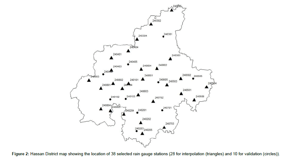
Figure 2: Hassan District map showing the location of 38 selected rain gauge stations (28 for interpolation (triangles) and 10 for validation (circles)).

Results and Discussıon

Pancreatic recovery depends on a perplexing communication between the cells that give vital recovery signals and cells that are responsive to those the signs. As talked about here, the level, nature and the seriousness of injury are three significant boundaries that decide whether recuperation is accomplished. β-cell recovery is shown to be more delicate to the idea of injury than the acinar recovery. At long last, the level of the injury figures out which cell types would react to these regenerative signs.

Data exploration

While annual rainfall values of all five years considered are more or less floating around the same mean, it is evident that 2012 has the lowest rainfall average of 930.67 mm and 2014 has the highest rainfall average of 1475.88 mm. The monthly rainfall for 5 years from 2011 to 2015 is also represented in the form of a bar graph Figure 3 to understand the seasonal variability in data. From Figure 4, it is clear that the peak rainfall occurs in the months of June/July or October. This is concordant with the seasonal rainfall variation in the region. A frequency table is developed for the monthly rainfall data, which is used to develop a histogram, indicative of the number of months in the span of 5 years that fall under a particular class of monthly average rainfall. Figure 4 shows that in 5 years, highest rainfall of greater than 300 mm occurs in July. In the span of 5 years, 25 months have rainfall between 0-45.81 mm and about 11 months have a monthly rainfall between 91.62-137.43 mm. These months primarily occur between December and May.

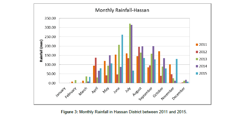
Figure 3: Monthly Rainfall in Hassan District between 2011 and 2015.

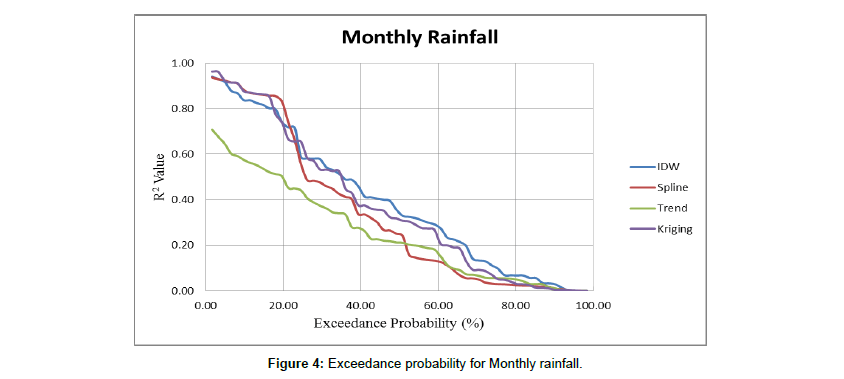
Figure 4: Exceedance probability for Monthly rainfall.

Interpolation using 5-year annual average rainfall

In order to capture the spatial variation of rainfall over Hassan District, 5-year annual rainfall averages for all the 28 rain gauge stations within the District were used to develop interpolated maps. All the interpolation techniques are based on the principle that closer things are more related than farther things. This principle yields different outcomes for different interpolation techniques owing to the variability in the different models that the techniques employ.

Considering the area of interest in the current study, it is known that rainfall increases as we move towards the south-western region of the Hassan District. This is due to the influence of “malnad” region in the District. Interpolation by IDW gives the effect of higher localised variation in rainfall around the actual points, as a result of assigning larger weight to validation points closer to it and a smaller weight to the points that are farther away. Spline interpolation produces gently varying surfaces where there is higher density of rain gauge stations. This is attributed to the fact that spline uses a regression equation to adapt the values at unknown points, by defining a radius around the measured point. The trend interpolator gives uniformly varying surfaces, using a linear mathematical function.

In order to indicate the level of concordance between the actual value and interpolated value, R² and RMSE values were computed for the chosen 10 validation points. The results of this computation are shown in Table 1.

Table 1: R²and RMSE values obtained for different interpolation techniques.

From Table 1, it is evident that the lowest RMSE value of 148.9 mm and higher R² value of 0.914 is obtained for spline interpolation. On the contrary, the least suitable method with the high RMSE of 364.6 mm and lowest R² value of 0.488 is obtained for trend interpolation. This can be attributed to the fact that the trend interpolation assumes a single polynomial to fit the sample points over the whole surface, thereby reducing the accuracy of the estimation. On the contrary, spline interpolation consists of a set of third-degree polynomials which describe pieces of lines or surfaces and they are fitted together to form a smooth surface. The ordinary kriging interpolator uses a spherical model and gives RMSE of 176.7 mm, which is similar to the RMSE obtained for IDW (173.6 mm). While the R² value gives an overall sense of how well the interpolated rainfall estimates correlate with the actual measured values, the RMSE tells us by how much our estimations deviate, on an average, from the actual values.

Interpolation of Monthly Rainfall

Monthly rainfall data obtained by adding daily rainfall over a month, for all 60 months spanning January, 2011 to December, 2015 were interpolated, facilitated through the Automated Rainfall Mapping Tool. Cross- validation results are tabulated in Tables 2 and 3. The R² and RMSE values reveal that all the techniques performed relatively better during the rainy months (June, July, August) by yielding low RMSE (22 mm to 150 mm) and high R² values (0.5 to 0.96), compared to the non-rainy months. The exceedance probability curve Figure 5 for all 60 months, indicates that for 10% of the total months considered, kriging and spline give R² of greater than 0.9, while for 50% of the total months considered, IDW performed better than the  other 3 methods, giving an R² value of 0.4. Trend interpolation technique appears to perform relatively poorly for all the months. Considering only the rainy months, it was noticed thatkriging, spline and IDW give R² values of more than 0.8 about 60% of the time Figure 6. While the three techniques appear to show similar behaviour at most of the times, one-on-one comparison indicate that kriging gives a R² value between 0.53- 0.96, spline takes on a value between 0.45-0.94 and IDW gives a value between 0.46 to 0.94. The exceedance curve Figure 6 for the rainy months shows that more than 70% of the time, kriging and IDW perform better than spline, with the two techniques showing very similar variation. However, performance of all 4 techniques degrades considering non-rainy months in the region Table 3. The exceedance probability curve Figure 7 shows that only for 10% of the time, the R² value reaches about 0.8 and for more than 50% of the time the R² value is less than 0.4. IDW and kriging have a relatively higher R² value compared to the other 2 techniques, for most part of the time period considered. A single technique does not consistently perform well for all months. This may be attributed to the highly variable nature of rainfall parameter and can also be due to the influence of topography and meteorological parameters.

Table 2: R² value and RMSE values obtained for different interpolation techniques, during the rainy months.

Table 3: R² value and RMSE values obtained for different interpolation techniques, during the non- rainy months.

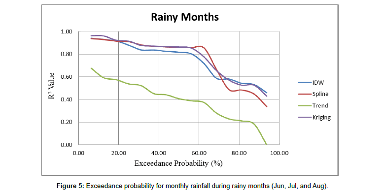
Figure 5: Exceedance probability for monthly rainfall during rainy months (Jun, Jul, and Aug).

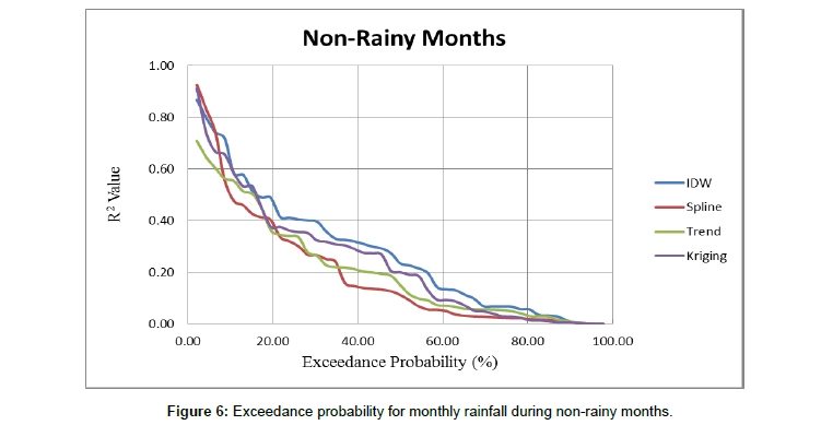
Figure 6: Exceedance probability for monthly rainfall during non-rainy months.

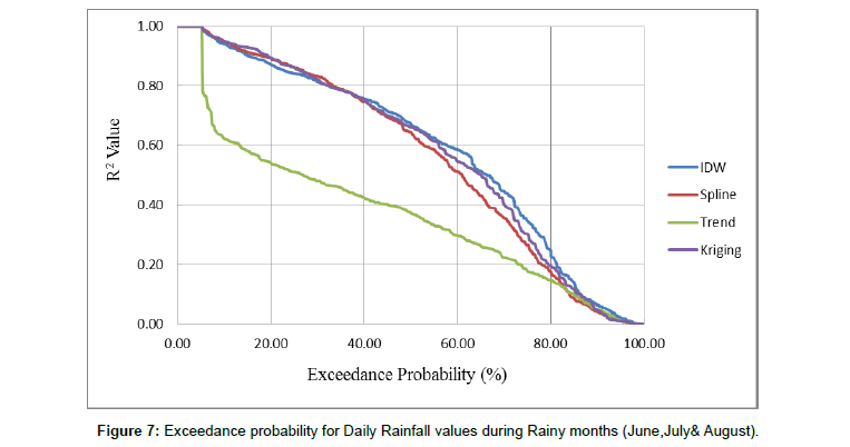
Figure 7: Exceedance probability for Daily Rainfall values during Rainy months (June,July& August).

Interpolation of daily rainfall during monsoon months

The exceedance probability for daily rainfall Figure 7 shows that throughout the time span considered, trend interpolator performed poorly compared to other techniques. IDW, spline and kriging are more or less homogeneous in their behaviour while interpolating the daily rainfall values during monsoon season. For 50% of the time, the 3 methods are alike and give R² value of 0.7, while trend gives R² value of 0.4. On considering more than 60% of the days, IDW and kriging have a relatively higher R² value of about 0.6, compared to spline and trend. The reason for IDW and kriging to perform better than spline may be attributed to the way the techniques model the spatial variability. IDW causes the interpolated value to be more similar to the measured value when it is close to it and the interpolated value decreases as we move farther away from the measured values, due to decrease in distance weights. Like IDW interpolation, kriging forms weights (which come from a semivariogram that is developed by viewing the spatial structure of the data) from surrounding measured values to predict values at unmeasured locations, where the closest measured values usually have the most influence. Spline performs a smoothing function to fit the measured points. It is a fairly well- established fact that kriging and IDW show maximum level of concordance for daily interpolation in the rainy months. During the non-rainy months, the techniques show large variability in their performance for each day and it is difficult to state definitively that one technique is best over the others.

Conclusion

The 5 years daily precipitation data for Hassan District from January, 2011 to December, 2015, was obtained from Karnataka State Natural Disaster Monitoring Centre (KSNDMC). Spatial interpolation by IDW, Trend, Spline and Ordinary Kriging (spherical model) method was carried out at temporal scales of 5 year annual average rainfall, monthly rainfall and daily rainfall data (only during the monsoon months - June, July and August), by considering 38 rain gauge stations (28 used for interpolation and 10 for validation). The Automated Rainfall Mapping tool was developed to facilitate interpolation at monthly and daily time scales, and to generate cross-validation results for the same. RMSE and R² values were used to assess the accuracy of the 4 interpolation techniques at the chosen temporal scales.

The analysis revealed that using spline technique gives best concordance to interpolate the 5-year annual average rainfall values over Hassan District, giving a RMSE of 148.9 and R² value of 0.914. Interpolation of monthly rainfall shows that even though a single technique does not perform well for all months, kriging, spline and IDW give R² greater than 0.8 for more than 60% of the time in the monsoon months, with kriging having higher R² range between 0.53 and 0.96. During the non-monsoon months, for more than 50% of the time, the R² value of all techniques is less than 0.4. It can be noted, however, that IDW and kriging perform relatively better than the other 2 techniques. Considering interpolated daily rainfall values during the monsoon season, although kriging, IDW and spline were identical in their performance for half the time, kriging and IDW gave higher R² value of about 0.6 for 60% of the days considered, compared with other 2 techniques.

During the non-rainy months, owing to the high variability in daily rainfall, a single method does not consistently perform well for each day.

Scope for Future Study

• A similar comparison of spatial interpolation techniques can be carried out for long-term rainfall data (Ex: 30 years precipitation data) so that it can be of use in climate studies and drought modelling.

• The automated rainfall mapping tool can be made dynamic to generate rainfall interpolation maps for each day, based on the value of error estimates for that day.

• The automated rainfall mapping tool can be made dynamic to generate rainfall interpolation maps for each day, based on the value of error estimates for that day.

The interpolated precipitation data and maps prove to be of paramount value in computing rainfall at ungauged locations, irrigation scheduling in agricultural fields and in the detection and prediction of changes in watersheds. Being region-specific, it is important to determine the validity of the interpolation techniques in different regions, as subsequent agricultural or hydrological decisions depend on the results obtained.

Acknowledgement

Authors acknowledge Karnataka State Natural Disaster Monitoring Centre (KSNDMC), Bengaluru for providing the rainfall data used in this study.

References

1. Piazza AD, Conti FL, Noto LV, Viola F, Loggia GL (2011) Comparative analysis of different techniques for spatial interpolation of rainfall data to create a serially complete monthly time series of precipitation for Sicily, Italy. Int J Applied Earth Observation and Geoinformation 13: 396-408.
2. Courault D, Monestiez P (1999) Spatial interpolation of air temperature according to atmospheric circulation patterns in southeast France. Int J Climatol 19: 365-378.
3. Apaydin HH, Kemal FS, Ersoy YY (2004) Spatial interpolation techniques for climate data in the GAP region in Turkey. Climate Research               28: 31-40.
4. Phillips DL, Dolph Jayne, Marks Danny (1992) A comparison of geostatistical procedures for spatial analysis of precipitation in mountainous terrain. Agric Forest Meteorology 58: 119-141.
5. Pandey V, Pandey PK (2010) Spatial and Temporal Variability of Soil Mositure. Int J Geoscience 1: 87-98
6. Zhang X, Srinivasan Raghavan (2009) GIS-based Spatial Precipitation Estimation: A Comparison of Geostatistical Approaches. Am J Water Resour 45(4): 894-906.
7. Dirks KN, Hay JE, Stow CD, Harris D (1998) High-resolution studies of rainfall on Norfolk Island Part II: Interpolation of rainfall data. J Hydrol 208: 187-193.
8. Ha W, Prasanna HG, Thomas O, Thomas HM, Dana O, et al., (2011) Spatial Interpolation of Daily Reference Evapotranspiration in the Texas High Plains. World Environmental and Water Resources Congress 2796-2804.
9. Robinson TP, Metternicht G (2005) Testing the performance of spatial interpolation techniques for mapping soil properties. Computer and Electronics in Agriculture 50: 97-108.
10. Hernández JJC, Gaskin SJ (2007) Spatio temporal analysis of daily precipitation and temperature in the Basin of Mexico. J Hydrol 336(3): 231-249.
11. Wagner PD, Fiener Peter, Wilken Florian, Kumar Shamita, Schneider Karl (2012) Comparison and evaluation of spatial interpolation schemes for daily rainfall in data scarce regions. J Hydrol 464(465): 388-400.
12. Luo W, Taylor MC, Parker SR (2008) A comparison of spatial interpolation methods to estimate continuous wind speed surfaces using irregularly distributed data from England and Wales. Int J Climatol 28: 947-959.
13. Mahalingam B, Amin Noori Deldar, Vinay M (2015) Analysis of Selected Spatial Interpolation Techniques for Rainfall Data. Int J cur Res Rev 7(7): 66-71.
14. Mukhopadhaya S (2016) Rainfall Mapping using Ordinary Kriging Technique: Case study: Tunisia. J Basic and Applied Engineering Research 3: 1-5.
15. Vincente-Serrano SM, Angel Saz-Sánchez M, José MC (2003) Comparative analysis of interpolation methods in the middle Ebro Valley (Spain): Application to annual precipitation and temperature. Climate Research 24: 161-180.
16. Goovaerts P (2000) Geostatistical approaches for incorporating elevation into the spatial interpolation of rainfall. J Hydrol 228: 113-129.
17. Frazier AG, Giambelluca Thomas W, Diaz Henry F, Needham Heidi L (2016) Comparison of geostatistical approaches to spatially interpolate month-year rainfall for the Hawaiian Islands. Int J Climatol 36: 1459-1470.