Research Article, Res Rep Math Vol: 2 Issue: 1

Extending the Applicability of an Ulm-Newton-like Method under Generalized Conditions in Banach Space

Ioannis K. Argyros^1* and Santhosh George²

Department of Forestry and Biodiversity, Tripura University, Suryamaninagar, Agartala, India

*Corresponding Author : Ioannis K. Argyros Department of Mathematical Sciences, Cameron University, Lawton, OK 73505, USA, E-mail: iargyros@cameron.edu

Received: November 02, 2017 Accepted: January 15, 2018 Published: February 10, 2018

Citation: Argyros IK, George S (2018) Extending the Applicability of an Ulm-Newton-like Method under Generalized Conditions in Banach Space. Res Rep Math 2:1

Abstract

Keywords: Ulm’s method; Banach space; local / semi-local conver-gence

Introduction

In this study we are concerned with the problem of approximating a locally unique solution x of equation

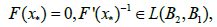
F (x) = 0; (1.1)

where, F is a Frechet{di erentiable operator de ned on a convex subset of a Banach space B1 with values in a Banach space B2.

A large number of problems in applied mathematics and also in engineering are solved by nding the solutions of certain equations. For example, dynamic systems are mathematically modeled by di erence or di erential equations, and their solutions usually represent the states of the systems. For the sake of sim-plicity, assume that a time{invariant system is driven by the equation x = R(x), for some suitable operator R, where x is the state. Then the equilibrium states are determined by solving equation (1.1). Similar equations are used in the case of discrete systems. The unknowns of engineering equations can be func-tions (di erence, di erential, and integral equations), vectors (systems of linear or nonlinear algebraic equations), or real or complex numbers (single algebraic equations with single unknowns). Except in special cases, the most commonly used solution methods are iterative{when starting from one or several initial approximations a sequence is constructed that converges to a solution of the equation. Iteration methods are also applied for solving optimization problems. In such cases, the iteration sequences converge to an optimal solution of the problem at hand. Since all of these methods have the same recursive structure, they can be introduced and discussed in a general framework [1-12].

Moser [13] proposed the following Ulm’s-like method for generating a sequence fxng approximating x :

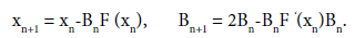
Method (1.2) is useful when the derivative F 0(xn) is not continuously invertible (as in the case of small divisors [1-8,10,11,13-15]). Moser studied the semi-localpconvergence of method (1.2) and showed that the order of convergence is 1 + 2 if F 0(x?) 2 L(B2; B1p). However, the order of convergence is faster than the Secant method (i.e. 2). The quadratic convergence can be obtained if one uses Ulm’s method [14,15]

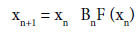
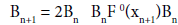
The semi-local convergence of method (1.3) has also been studied in [1-9]. As far as we know the local convergence analysis of methods (1.2) and (1.3) has not been given. In the present paper, we study the local convergence of the Ulm’s-like method de ned for each n = 0; ; 2; 3; : : : by

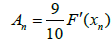
where A_n is an approximation of F’(x_n). Notice that method (1.4) is inverse free, the computation of F⁰(x_n) is not required and the method produces suc-cessive approximations {B_n} ≈ F’(x*)^-1

In Section 2, we present the local convergence analysis of the method (1.4) and in Section 3, we present the numerical examples.

Local convergence analysis

The local convergence analysis of the method (1.4) is given in this section. Denote by U (v, ζ) the open and closed balls in B₁, respectively, with center v ∈ B₁ and of radius ζ>0.

Let w₀ : [0,+ ∞] → [0,+ ∞] and w : [0,+ ∞] →[0,+ ∞] be continuous and nondecreasing functions satisfying w₀ (0)= w(0)=0.

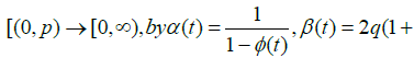
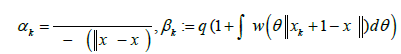
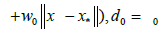
Let also q ∈ [0,1] be a parameter. Define functions Ï�? and ψ on the interval [0,+ ∞] by

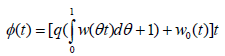
and

We have that ψ (0) = −1 and for sufficiently large 0 0 t ≥ t,ψ (t ) > 0 . By the intermediate value theorem equation ψ (t) = 0 has solutions in the interval (0, t₀). Denote by the smallest such solution. Then, for each t ∈[0,ρ ]we have

0 ≤ψ (t) < 1. (2.1)

We need to show an auxiliary perturbation result for method (1.4).

LEMMA 2.1 Let be a continuously Frechet-differentiable operator. Suppose that there exist , continuous and nondecreasing functions and such that for each x∈Ω,n = 0,1,2,.. and θ ∈[0,1]

that for each

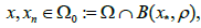
where

and

where

Then, the following items hold

And

Proof we shall first show estimate (2.11) holds. Using (2.1), we have the identity

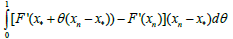(2.14)

Then, by (2.4) and (2.14) we have that

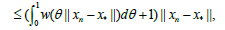
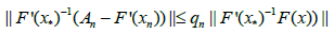
which shows (2.10). Moreover, by (2.5), (2.6) and (2.10) we obtain that

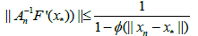
which shows the estimate (2.11). Furthermore, using (2.3), (2.4), (2.10), (2.11) and the definition of r₀ we get that

(2.15)

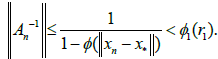
It follows from (2.15) and the Banach lemma on invertible operators [1,4,6,11] that (2.12) and (2.13) hold.

REMARK 2.2 In earlier studies the Lipschitz condition [1-15]

(2.16)

is used which is stronger than our conditions (2.3) and (2.4). Notice also that since

(2.17)

and

(2.18)

where functions w₁ is as function w but defined on Ω instead of Ω₀.The ratio can be arbitrarily large [1,4,6]. Moreover, if (2.16) is used instead of (2.3) and (2.4) in the proof of Lemma 2.1, then the conclusions hold provided that r0 is replaced by r1 which is the smallest positive solution of equation

(2.19)

where it follows from (2.10), (2.17), (2.18), (2.19) that

Furthermore, strict inequality holds in (2.20), if (2.17) or (2.18) hold as strict

Inequalities. Finally, estimates (2.11) and (2.12) are tighter than the corresponding ones (using (2.16)) given by

Let λ be a parameter satisfying be a continuous and no decreasing function.

Moreover, define functions

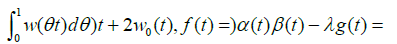
Parameters and quadratic equatio Then, we have

Denote byρ₀ the smallest solution of equation f(t)=0 in (0,p) tthen, we have

that for each

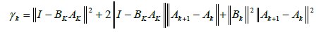
In view of the above inequality the preceding quadratic equation has a unique positive solution denoted by ρ+ and a negative solution. Define parameter γ by

Then, we have that

Notice that we also have that and

Next, we present the local convergence of method (1.4).

THEOREM 2.3 Under the hypotheses of Lemma 2.1 and with r0 given in (2.9) for λ ∈[0,1) further suppose there exists function 2 0 w :[0,r )→[0,+∞) continuous and no decreasing such that for each and

for each

and

where γ is given in (2.22). Then, sequence generated by the method (1.4) for is well defined , remains in * B(x ,γ ) and converges to x*

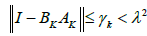
Proof. We have by hypothesis (2.25) that so

is true for k = 0: Suppose that (2.27) is true for all integers smaller or equal to k: Using Lemma 2.1, we have the estimate

In view of method (1.4) for n = k; we can write in turn that

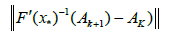
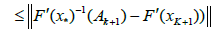
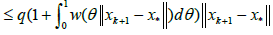
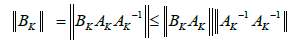
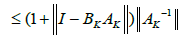
By the definition of method (1.4), we have the estimate

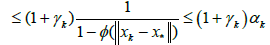
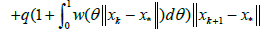
Then, by (2.32), (2.29) for n = k; we get in turn that

which shows (2.27) for n = k +1: Then, using the induction hypotheses, (2.24), and the definition of γ

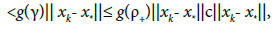
where c = g[0,1], so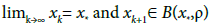

REMARK 2.4 (a) As noted in Remark 2.2 conditions (2.4) and (2.5) can be replaced by (2.24).

(2.36)

for each x∈Ω and θ ∈[0,1], where function ω₃is as ω₁:

We have that ω₁ (t)≤ ω₃ (t). Then, in view of Remark 2.2 and (2.24) the radii of convergence as well as the error bounds are improved under the new approach, since old approaches use only (2.36) with the exception of our approach in [2,5].

The results obtained here can be used for operators F satisfying autonomous differential equations [1,4,6,11] of the form

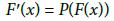
Where is a continuous operator. Then, since F′(x*)= P(F(x*))= P(0), we can apply the results without actually knowing x* For example, let F(x) =ex^-1. Then, we can choose P(x) = x + 1

(c) The local results obtained here can be used for projection methods such as the Arnoldi’s method, the generalized minimum residual method (GM-RES), the generalized conjugate method (GCR) for combined Newton/finite projection methods and in connection to the mesh independence principle can be used to develop the cheapest and most efficient mesh refinement strategies [1,4,6].

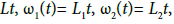
(d) Let L₀, L, L₁, L₂, L₃ be positive constants. Researchers, choose ω₀(t)= L₀t, ω(t)= Lt, ω₁(t)= L₁t, ω₂(t)= L₂t, and ω₃(t)= L₃t, Moreover, if we choose Ω₀=Ω and L=L₁ then, our results reduce to the ones given by where the second order of convergence was shown with the Lipschitz conditions given in non-affine invariant form. In Example 3.1, we shall show that the radii are extended and the upper bounds on ||x_n- x*|| are tighter if we use ω₀, ω, ω₂ instead of using ω₀ and ω we used in [5] or only ω3 as used in [2,7-15].

Numerical examples

Example 3.1 let 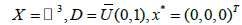Define function F on D for ω=(x,y,z)^T by

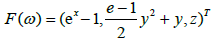
Then, the Frechet-derivative is defined by

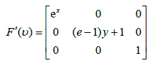
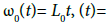
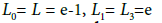Notice that using the Lipschitz conditions, we get and where and Moreover, choose to obtain

The parameters are

where the bar answers corresponding to the case when only ω₃ is used in the derivation of the radii.

Example 3.2 Let

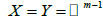for natural integer

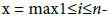
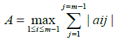
X and Y are equipped with the max-norm The corresponding matrix norm is

For 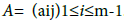On the interval [0; 1], we consider the following two point boundary value problem

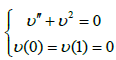(3.1)

[6,8,9,11]. To discretize the above equation, we divide the interval [0; 1] into m equal parts with length of each part: h=1/m and coordinate of each point: x_i=I h with i=0,1,2,…,m. A second-order finite difference discretization of equation (3.1) results in the following set of nonlinear equations

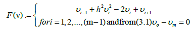(3.2)

Where 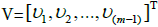For the above system-of-nonlinearequations, we provide the Frechet derivative

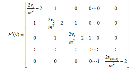
We see that for

where 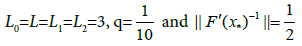The parameters are

where the bar answers corresponding to the case when only ω3 is used in the derivation of the radii.

References

1. Argyros IK (2007) Computational Theory of Iterative methods. Elsevier Publ. Comp. New York.
2. Argyros IK (2009) On Ulm's method for Frechet differentiable operators.J Appl Math Computing 31: 97 - 111.
3. Argyros IK (2009) On Ulm's method using divided differences of order one. Numer. Algorithms 52: 295-230.
4. Argyros IK, Hilout S (2014) Computational Methods in Nonlinear Analysis - Efficient Algorithms, Fixed Point Theory and Applications, World Scientific.
5. Argyros IK (2014) On an Ulm's -like method under weak convergence conditions in Banach space. Advances in Nonlinear Variational Inequalities 2: 1-12.
6. Argyros IK, Magrenan AA (2017) Iterative methods and their dynamics with applications, CRC Press, New York.
7. Burmeister W (1972) Inversionsfreie Verfahren zur L•osung nichtlinearer Opera-torgleichungen, ZAMM 52: 101-110.
8. Ezquerro JA, Hernandez MA (2008) The Ulm method under mild differentiability conditions, Numer. Math. 109: 193-207.
9. Gutierrez JM, Hernandez MA, Romero N (2008) A note on a modi cation of Moser's method, Journal of Complexity, 24: 185-197
10. Hald OH (1975) On a Newton-Moser-type method, Numer. Math. 23: 411-426.
11. Kantorovich LV, Akilov GP (1982) Functional Analysis, Pergamon Press, Ox-ford Publications, Oxford.
12. Moret I (1987) On a general iterative scheme for Newton-type methods, Numer Funct Anal Optim 9: 1115-1137.
13. Moser J (1973) Stable and random motions in dynamical systems with special emphasis on celestial mechanics. Herman Weil lectures, Annals of Mathe-matics Studies, Princeton University Press, Princeton, NJ.
14. Ulm S, Das Majorantenprinzip und die Sehnenmethode (Russ.), Izv Akad Nauk Est SSR 13: 217-227.
15. S. Ulm (1967) Uber Iterationsverfahren mit suksessiver Approximation des in-versen Operators (Russ.), Izv Akad Nauk Est SSR 16: 403-411.