Spanish
  Chinese
  Russian
  German
  French
  Japanese
  Portuguese
  Hindi
Hindi Research Article, Geoinfor Geostat An Overview Vol: 6 Issue: 2
Fusion Based on Geostatistics to Improve the Altimetry Accuracies of Digital Elevation Models
Felgueiras CA*, Ortiz JO, Camargo ECG, Namikawa LM, Rosim S, Oliveira JRF, Renno CD, Sant’Anna SJS and Monteiro AMV
INPE, Brazilian National Institute for Space Researches, Sao Jose dos Campos, Sao Paulo, Brazil
*Corresponding Author : Felgueiras CA
INPE, Brazilian National Institute for Space Researches, Sao Jose dos Campos, Sao Paulo, Brazil
Tel: +5512980000000
E-mail: carlos@dpi.inpe.br
Received: March 30, 2018 Accepted: April 23, 2018 Published: May 03, 2018
Citation: Felgueiras CA, Ortiz JO, Camargo ECG, Namikawa LM, Rosim S, et al. (2018) Fusion Based on Geostatistics to Improve the Altimetry Accuracies of Digital Elevation Models. Geoinfor Geostat: An Overview 6:2. doi: 10.4172/2327-4581.1000179
Abstract
Fusions based on geostatistical methods are used in this article to improve the accuracy of the altimetry attribute of Digital Elevation Models (DEMs). Ordinary kriging, kriging with external drift, regression kriging and cokriging procedures, are applied to assess uncertainty representations from which it is possible to get altimetry predictions and other information. The fusion data modeling is performed from existing DEMs, mainly available for free in the internet, and additional high accurate set of 3D sample points. Although the freeware DEMs are dense and generally have good spatial distributions, the accuracy of their altimetry information
might not be suitable for many applications. A way of mitigating this problem is to combine, in the data modeling processes, the available DEM data along with additional information coming from various other sources and having better quality. Usually, high accurate altimetry data are collected in field works, with higher cost,
at specific point locations inside the spatial region of interest. In short, this work aims to integrate, through geostatistical methods, spatial elevation information of different sources, data structures and elevation accuracies to obtain better accurate DEMs. The methodology addressed in this research was applied to a case
study in a Brazilian Southeast geographical region. Quantitative and qualitative validations were performed using an independent high accurate data set and comparisons based on DEM differences and drainage network automatic extraction. For the considered study area, the kriging with external drift and the regression kriging have led to similar quantitative and qualitative improvements, better than the co-kriging approach.
Keywords: Elevation data fusion; Digital elevation modeling; DEM accuracy; Geostatistics; Kriging; Co-kriging
Introduction
Digital Elevation Models (DEMs) are applied in a large number of geographic environmental applications, such as, agriculture, geology, cartography, hydrology, rural and urban planning, among others [1]. DEMs are digital topographic information usually represented as spatial rectangular grids that are very suitable to be used in Geographical Information Systems (GISs) applications. Many derived products can be attained directly from DEMs as, for example, slope and aspect maps, drainage networks, contour lines, and profile and volume calculations [2]. Also, spatial modeling, developed in GIS environments, frequently uses DEMs, or their derived products, as input information. Nowadays it is possible to obtain DEM information for free, in the internet with no financial costs, of almost every region of the earth surface. Although these DEMs are dense and generally have good spatial distributions, the accuracy of their vertical information, the altimetry, might not be suitable for many applications. A way of mitigating this problem is to combine the available DEM data along with other information, coming from more reliable sources and having better quality, in the data modeling processes. Elevation information of the earth surface can be also obtained as a set of spatial locations, 3D points, sampled in a geographical region of interest. These samples can be collected with very high vertical accuracy using Global Positioning System (GPS) equipment, for example.
Geostatistical tools have been extensively used to analyze and to model environmental attributes represented as a set of sample points of geophysical and geochemical indices, concentrations of soil elements, elevations, temperatures, etc. [3-5]. Some geostatistical procedures allow performing conflations by combining different sources of environmental attributes [6-13]. Geostatistical procedures known as kriging and simulation can be used to integrate existing DEMs with sample points of altimetry of the same geographical region. In short, this integration aims to obtain a more accurate derived DEM than the original one.
In this context, the objective of this article is to explore and analyze geostatistical methods to perform fusions of existent DEMs with sample set of elevation points to obtain more accurate results on modeling the altimetry information. It is considered that the points of the sample set, here referred as hard or primary data, have higher vertical accuracy than the original DEM, here called soft or secondary data. The geostatistical procedures, Ordinary Kriging (OK), Kriging with External Drift (KED), Regression Kriging (RK) and CoKriging (CoK), are considered to perform the fusions. A case study is presented with data from a Brazilian Southeast geographical region to illustrate the application of the proposed methodology. For the fusions on the region of the case study it was used a Shuttle Radar Topography Mission (SRTM) DEM and a set of high accurate sample points. Quantitative validations are assessed with statistics and Root Mean Squared (RMS) metrics using an independent hard sample set. Also, qualitative analyzes are performed comparing DEMs differences and drainage maps automatically extracted from the elevation models.
Basic Concepts
Kriging
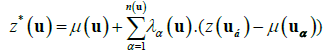
Kriging is a geostatistical technique used for estimations of spatial attributes (elevations, in this work) at locations not previously sampled from a set of sample points. The Kriging is known as a BLUE (Best Linear Unbiased Estimation) estimator. The kriging procedure allows to infer a mean value z*(u) of the attribute, at any spatial location u, from a number n(u) of neighbor samples z(uα), α=1, 2,..., n(u). The general formulation for the geostatistical kriging estimator is defined by Deutsch et al. [14], Isaaks et al. [3] as
 (1)
(1)
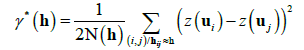
where μ(u) is the mean, or the expected value, of the attribute in the spatial location u and μ(uα) is the mean value at each sampled location uα. The kriging weights λα(u) are constrained to sum to 1 and are assessed considering the correlation structure defined by a modeled semivariogram gotten from the total set of n sample points considered. Empirical, or experimental, semivariograms, γ*(h), can be estimated, directly from a set of sample points, according to:
 (2)
(2)
where z(ui) and z(uj) are attribute values observed at sampled spatial locations ui and uj separated by the distance h. N(h) is the number of samples found inside a circumference with radius distance approximately equal to h. Mathematical, or conceptual, semivariograms are then fitted for the empirical ones to be used in the evaluation of the kriging weights of Equation 1. Typically, spherical, exponential, gaussian and power mathematical models are considered in the fitting process.
Kriging with external drift
The KED approach is a kriging considering a trend model. The trend is obtained from a secondary variable related to the primary one. The trends are used as the mean values, in the Equation 1, and the residual covariance, rather than the covariance, of the primary variable must be used to solve this kriging approach.
Deutsch et al. [14], point out two conditions that have to be met before applying the external drift algorithm: (1) The external variable must vary smoothly in space and (2) The external variable must to be known at all locations uα of the primary data and at all locations u to be estimated. The advantage in this case is that it is not necessary to know the cross covariance between the primary and secondary variables. In this work the input DEM is considered the external drift yelling elevation data at all locations of the condition (2) above.
Regression kriging
The Regression Kriging (RK) interpolation is based on regression of the primary variable on spatially exhaustive secondary information. The predictions are made by modelling the relationship between the target (primary) and auxiliary (secondary) variables at sample locations and applying it to unvisited locations using the known value of the auxiliary variables at those locations [7]. The RK combines these two approaches: Regression of Ordinary or Generalized Least Squares (OLS or GLS) can be used to fit the explanatory variation and simple kriging, with expected value 0, is used to fit the residuals, i.e. unexplained variation [6]. The general formulation for the RK estimator is:
Z*(u) = μ(u) + e*(u)
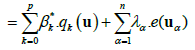 (3)
(3)
where μ(u) is the fitted drift, e*(u) is the interpolated residual, β*k are estimated drift model coefficients, λα are simple kriging weights and e(uα) is the residual at location uα
Equation 3 points out that the z* estimated value at any spatial location u is evaluated by summing the trend component, resulted from the fitted regression, with the simple kriging of the residuals. Comparison of KED and RK geostatistical methods is addressed by Hengl et al. [15].
Cokriging
The geostatistical cokriging procedure allows to incorporate a secondary variable Y, besides the primary Z one, into the kriging estimator process. The ordinary cokriging (CoK) estimator at spatial location u for two random variables, Z and Y with values known at locations uα1 and uα2 respectvely, is written as Goovaerts et al. [4].
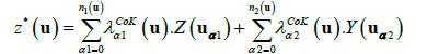 (4)
(4)
with the CoK weights of the primary variable  constrained to sum to one and the CoK weights of the secondary variable
  constrained to sum to zero.
The cokriging is a more complex geostatistical technique since requires the computing and modelling of three semi-variograms related to the Z and Y random variables, two directs and one cross semi-variogram. The KED and RK approaches, above presented, are alternative techniques that overcome the CoK complexity by requiring the evaluation of only the primary semi-variogram.
Drainage extraction from DEMs
Drainage network is an important computational product to simulate water behavior in hydrographic basins. It basically depends on the drainage extraction method used, on the quality of the altimetry data and on the resolution of this data, which must be adequate to the work scale. There are many methods to obtain automatically the drainage network from a DEM data. For example, in the TerraHidro application by Rosim et al. [16] the drainage network system extraction is automatically performed by the following steps using an altimetry regular grid [17]: (1) local flow extraction determining the direction of greatest slope relative to its 8 grid neighbors; (2) calculation of area contribution creates a new grid where each grid cell contains the value of its area multiplied by the number of cells through which the water passes until it reaches this cell; (3) drainage network determination which defines a particular drainage by providing a threshold value relative to the contributing area, creating a new grid (all cells in the contribution area grid, with values equal to or greater than the given threshold, will be flagged as drainage cells in the drainage grid); (4) drainage network vectorization, if necessary.
Validations of DEMs and their Products
Quantitative validations
The quantitative validations of the grids are performed using an independent validation sample set with vertical high accuracy. The validation sample values zv are compared, at same spatial position uα with the grid values zg and statistics, as the mean error em and the standard deviation error estd are evaluated for the n samples as:
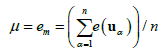 (5)
(5)
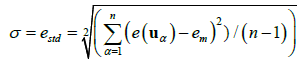 (6)
(6)
where, e(uα)= zg (uα)- zv (uα)is the local error at the sampled spatial location,
The Pearson correlation ρ is also considered:
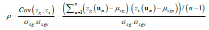 (7)
(7)
In addition, the RMS error eRMS value is calculated for the validation sample:
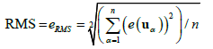 (8)
(8)
Qualitative validations
The qualitative validations can be accomplished making comparisons among DEM derived products, as contour lines or drainage networks, with the actual shapes. Generally, the derived products are overlaid on the actual shapes, using different colours for example, and visual analyses are performed for the comparisons. Also, visual and global statistical comparisons can be also performed on maps resulting from the difference between the fused DEMs and the input DEM used as reference.
Methodology
The methodology of this work has the following steps:
1. Create a database for a geographic region of interest in a GIS with basic information: a SRTM data and a set of sample points of high accurate elevations.
2. Perform spatial data exploratory analysis of the basic information.
3. Extract the trends of the basic information creating residual stationary information.
4. Assess the spatial variation of the residuals through direct and cross semi-variograms, empirical and conceptual.
5. Apply the Ordinary Kriging procedure in the sample set of elevations using its conceptual semi-variogram.
6. Assess the SRTM collocated elevation values related to the spatial position of the sample set of elevations. This was performed using bilinear interpolation over the SRTM grid cells.
7. Apply the KED, RK and CoK procedures using the SRTM and the sample set of elevations generating the fused DEMs
8. Use an independent sample set of elevation points for making quantitative validations and analyses of the SRTM and the fused maps using statistics and RMS metrics.
9. Generate and analyse maps of differences between the fused DEMs and the SRTM
10. Extract drainage networks from the SRTM, KED, RK and CoK grids
11. Perform comparative analyses of the drainage networks with actual drainage features extracted from a high resolution remote sensing image of the studied region
Case Study
As a case study, the above methodology was applied to a geographic region located in a Brazilian Southeast geographical region, known as Jacarei, state of Sao Paulo. The studied region has the following geographical bounding box: w 46o 4’ 4.98’’ to w 46o 0’ 2.82’’ and s 23o 16’ 2.91’’ to s 23o 12’ 47.23’’. Figure 1 shows the geographical location of the region considered in this case study.

Figure 1: Geographical location of the study area.
Figure 2 shows the spatial distribution of the input data: the SRTM and the set of sample points of the region of interest. The samples are the hard or primary variable while the SRTM is the soft or secondary one. It was used 406 sample points, blue marks in the Figure 2, for interpolation and 40 sample points, red marks in Figure 2, for validation purposes.

Figure 2: Input data: (a) SRTM and (b) set of sample points of the study geographical region.
The set of sample points have approximately 0.1 m of height accuracy while the SRTM RMS height accuracy is about 5.5 m, value assessed from the validation sample set. The SRTM elevations vary between 560.0 m and 794.9 m, with mean value equal to 682.9 and standard deviation equal to 43.3 m. The set of 406 elevation samples vary between 557.0 m and 779.7.9 m, with mean equal to 609.9 and standard deviation equal to 39.3 m.
It was used the SPRING GIS (Camara et al. [18], Camargo et al. [19]), the GsLib (Deutsch et al. [14]), the statistical R language (R Core Team [20]) and the TerraHidro (Rosim et al. [16]) software’s to develop the proposed methodology for this case study.
Results and Analysis
Estimation results
Direct and Cross semi-variograms from the residuals of the SRTM and from the set of 406 sample points are depicted in Figure 3.

Figure 3: Direct and Cross semi-variograms of the (a) set of 406 sample points, (b) SRTM and (c) set of 406 sample points plus SRTM.
The SRTM semi-variogram was obtained using its grid values based on the collocated 406 hard samples and by means of bilinear interpolation. Based in the graphics of Figure 3, Table 1 reports the parameters of the conceptual semi-variograms used in this work. In that table, Hard and Soft are the direct semi-variograms of the primary and secondary variables while Hard x Soft is their crossed semi-variogram. The semi-variogram structures show that the hard data has more variability, greater sill and range values, while soft data presents is more homogeneous. The determinants of the nugget coefficients and the exponential structure factors, sill and range, were checked for lead to a positive definite covariance model [14].
| Semi-variogram | Model | Nugget (m) | Sill (m) | Range (m) |
|---|---|---|---|---|
| Hard | Exponential | 1 | 462 | 776 |
| Soft | Exponential | 1 | 389 | 948 |
| Hard x Soft | Exponential | 0 | 406 | 862 |
Table 1: Parameter of the conceptual semi-variograms of Figure 3.
Figure 4 illustrates estimated maps resulting from (a) OK applied only to the set of 406 sample points, and from (b) KED applied to the set of 406 sample points along with the SRTM data as the external drift. Figure 5 shows estimated maps from (a) RK applied to the set of 406 sample points along with the SRTM data and from (b) CoK procedure applied the 406 sample points, considered as primary variable, and the SRTM, as secondary variable. Table 2 reports some statistical values of the DEMs presented in Figures 4 and 5.
| Min (m) | Max (m) | Mean | Median | Std. Dev. | |
|---|---|---|---|---|---|
| SRTM | 560.05 | 794.92 | 622.87 | 614.46 | 43.30 |
| OK | 557.48 | 778.25 | 617.54 | 607.93 | 37.24 |
| KED | 552.81 | 786.11 | 621.28 | 611.98 | 44.38 |
| RK | 555.04 | 800.05 | 621.52 | 612.80 | 44.62 |
| CoK | 555.11 | 800.96 | 623.90 | 615.69 | 44.11 |
Table 2: Statistics of the DEMs considered in the methodology of this work.

Figure 4: Estimated maps using (a) Ordinary Kriging applied to the set of 406 sample points and (b) Kriging with External Drift applied to the SRTM and the set 406 sample points of the study region.

Figure 5: Estimated maps using (a) Regression Kriging and (b) Cokriging maps applied to the SRTM and the set 406 sample points of the study region
A visual analyze of the maps of Figures 4 and 5 shows that the integration of the SRTM with the hard sample set allows to obtain a more detailed map than the one that was predicted only with the set of 406 sample points. Moreover, although the visual comparison of the SRTM, KED, RK and CoK maps leads to consider them very similar, or even equals, the statistical values reported in Table 2 show that they have similar statistical values but they are different.
Quantitative and qualitative validations
Tables 3 and 4 report some quantitative metrics, statistics and RMS values, related to the accuracy of the resulting predicted maps validated by the set of 40 independent sample points. Table 3 reports percentage of the Standard Deviation (Std Dev) and RMS improvements relative to their correspondent SRTM values, 5.24 m and 5.49 m, while in the Table 4 the improvements are relative to their correspondent OK values, 8.48 m and 8.40 m.
| Estimator | Mean (m) |
Std. Dev. (m) |
Correlation | RMS (m) |
StdDev Improv. (%) |
RMS Improv. (%) |
|---|---|---|---|---|---|---|
| SRTM | 1.84 | 5.24 | 9.90*10-1 | 5.49 | 0 | 0 |
| KED | 0.78 | 3.77 | 9.95*10-1 | 3.80 | 28.05 | 30.78 |
| RK | 0.82 | 3.82 | 9.94*10-1 | 3.85 | 27.10 | 29.87 |
| CoK | 2.88 | 4.75 | 9.91*10-1 | 5.50 | 9.35 | -0.18 |
Table 3: Validation results with Std Dev and RMS improvements (Improv.) relative to the correspondent SRTM values.
| Estimator | Mean (m) |
Std. Dev. (m) |
Correlation | RMS (m) |
Std Dev Improv. (%) |
RMS Improv. (%) |
|---|---|---|---|---|---|---|
| OK | 0.68 | 8.48 | 9.72*10-1 | 8.40 | 0 | 0 |
| SRTM | 1.84 | 5.24 | 9.90*10-1 | 5.49 | 38.21 | 34.64 |
| KED | 0.78 | 3.77 | 9.95*10-1 | 3.80 | 55.54 | 54.76 |
| RK | 0.82 | 3.82 | 9.94*10-1 | 3.85 | 54.95 | 54.17 |
| CoK | 2.88 | 4.75 | 9.91*10-1 | 5.50 | 43.99 | 34.52 |
Table 4: Validation results with Std Dev and RMS improvements (Improv.) relative to the correspondent Ordinary Kriging values.
In a qualitative visual analyzes it is very difficult to perceive differences comparing the DEM of the Figure 2 and the fused DEMs of Figures 4 and 5. Even the Pearson correlation, reported in Table 3, are greater than 99 percent, which explains why they show resemblance one to another. However, the quantitative validation results presented in Tables 3 and 4 show an improvement in the precision of the fused DEMs since their Std Devs are lower than the SRTM one. Nevertheless, the CoK DEM has a mean value much greater than zero, showing a biased outcome of the method, which leads to a higher RMS value.
From these Tables 3 and 4 it can also be observed significant percentages of improvements in Std Dev and RMS accuracies for the KED and RK estimators. Therefore, the reported quantitative validations demonstrate that, in this experiment, the KED and the RK have similar results and they perform better than the CoK considering the percentage of Std Dev and RMS accuracy improvements.
Figure 6 presents maps of differences between the derived DEM and the SRTM DEMs (KED-SRTM, RK-SRTM and CoK-SRTM). The hard samples were overlaid on the maps to assist analysis. Instead of global information, these maps allow to observe the spatial distribution of the differences. Blue regions mean negative differences where the SRTM elevation values are greater than the fused DEM. Green regions represent more similar values while the red ones show SRTM elevation values smaller than the derived DEM.

Figure 6: Maps of difference between the (a) KED, (b) RK and (c) CoK DEMs and the SRTM DEMs.
From these figures one can perceive that the upper left corner presents concentration of greater differences, mainly in the map (a) of Figure 6. Greater blue regions also appear in this same map, which leads to the perception that the KED approach performs greater local modifications in the original SRTM. As it is expected, it can be noted that, in general, regions with no hard samples are pictured with green hues meaning that the SRTM was not modified in these areas.
Table 5 reports extreme values, minimum and maximum, and global statistics of the maps of Figure 6. Analyzes considering the results of Figure 6 and Table 5 show more heterogeneity, greater standard deviation and greater difference between maximum and minimum values, in KED-SRTM than in RK-SRTM which, in turn, are greater than in CoK-SRTM map. This means that the original SRTM was less modified by the CoK procedure. These results agree with the quantitative validation presented in the Table 1. Figure 6 shows also that the greater positive differences are more concentrate in the upper left side of the study region.
| Minimum (m) |
Maximum (m) |
Mean (m) |
Median (m) |
Std Dev (m) |
|
|---|---|---|---|---|---|
| KED-SRTM | -23.96 | 19.55 | -1.59 | -1.85 | 4.92 |
| RK-SRTM | -22.92 | 16.30 | -1.35 | -1.48 | 3.07 |
| CoK-SRTM | -22.52 | 17.02 | 1.03 | 1.04 | 1.86 |
Table 5: Extreme values and statistics of the differences presented in the maps of figure 5.
Figure 7 illustrates a reference drainage map, blue line that was manually digitalized from a high resolution remote sensing image of the considered region. It was used a Rapid Eye multispectral image (MMA [21]), taken on Nov/02/2013, having spatial resolution of 5 m and a colored composition associating the bands 5, 3 and 2 to the red, green and blue color levels. The study region is crossed by a main river, called Parateí, along with minor streams directly, or indirectly, connected with it. Because the connected streams are too small and hard to be identified in the image, in this work only the main river was considered as reference drainage information [22].

Figure 7: Rapid Eye Image of the study area highlighting the Parateí River.
Also, drainage maps were automatically extracted from the SRTM and the fused DEMs. Figure 8 depicts the drainage network, extracted from the (a) SRTM, (b) KED, (c) RK and (d) CoK DEM models and the hard sample points, green marks, overlaid on the Rapid Eye image.

Figure 8: Drainage network extracted from the (a) SRTM (dark blue), (b) KED (cyan), (c) RK (yellow) and (d) CoK (pink) DEM models.
A general visual analyzes of the drainage lines of Figure 8, considering the Parateí river as the reference, show that the lines agree, or are very close, in most of the spatial locations. There are also some regions where they disagree, mainly where the land cover is composed by dense and high vegetation, as for example, the black square regions in Figure 8. Also, the lack of hard samples did not allow capturing the drainage streams at these regions.
It can also be observed that in some areas, as for example inside the highlighted ellipse regions in Figure 8, because of the presence of hard samples, the extracted lines of the fused DEMs appear closer to the Parateí river. Although the CoK extracted lines do not change significantly inside these regions.
Conclusions
This work explored some geostatistical procedures that allow fusing elevation data obtained from different sources and having different representation and height accuracy. It was considered the KED, RK and CoK geostatistical methods to obtain, in a case study, elevation predictions by integrating SRTM data with a set of high accurate set of sample points. Quantitative validations were assessed by statistics and RMS metrics using an independent hard sample set of points. Also, qualitative analyzes were performed comparing DEMs differences and drainage maps extracted from the elevation models.
The quantitative results of the validations showed improvements in the accuracy of the final fused DEM products for the study area. The KED and RK yielded similar quantitative results and better than the CoK procedure. Therefore, the experiment demonstrated that is possible to improve the accuracy of existing DEMs by the geostatistical tools considered in this work. Also, qualitative analyzes were performed showing that visually better derived products, as drainage maps for example, can be obtained from the fused DEMs.
In the future we intend to explore other geostatistical procedures that allow the combination of the two types of elevation data representations used in this work. Also, other derived products, as slope or convexity maps, for example, could be considered to evaluate the qualitative improvements of the fused DEMs.
Acknowledgements
The authors would like to thank FAPESP -the Sao Paulo Research Foundation-for the support obtained, via process number 2015/24676-9, to develop the researchers reported in this article.
References
- Maune DF, Nayegandhi A (2007) Digital Elevation Model. Technologies and Applications: The DEM User’s Manual. American Society for Photogrammetry and Remote Sensing Press. Minnesota University, Minneapolis, USA.
- Burroughs PA (1987) Principles of geographical information systems. Oxford University Press, New York, USA.
- Isaaks EH, Srivastava RM (1989) An introduction to applied geostatistics. Oxford University, New York, USA.
- Goovaerts P (1997) Geostatistics for natural resources evaluation. Oxford University Press, New York, USA.
- Wackernagel H (1998) Multivariate Geostatistics. Springer, New York, USA.
- Hengl T, Heuvelink GBM, Stein A (2004) A generic framework for spatial prediction of soil variables based on regression-kriging. Geoderma 120: 75-93.
- Hengl T, Heuvelink GBM, Rossiter DG (2007) About regression-kriging: From equations to case studies. Computers & Geosciences 33: 1301-1315.
- Hengl T, Bajat B, Blagojevic D, Reuter HI (2008) Geostatistical modeling of topography using auxiliary maps. Computers & Geosciences 34: 1886-1899.
- Karkee M, Steward BL, Azis SA (2008) Improving quality of public domain digital elevation models through data fusion. Biosystems Engineering 101: 293-305.
- Kyriakidis PC, Shortridge AM, Goodchild MF (1999) Geostatistics for conflation and accuracy assessment of digital elevation models. International Journal of Geographical Information Science, 13: 677-707.
- Felgueiras CA, Ortiz JO, Camargo ECG (2014) Application of Geostatistical Conflation Techniques to Improve the Accuracy of Digital Elevation Models. XV Brazilian Symposium on Geoinformatics, Campos do Jordão, São Paulo, Brazil.
- Felgueiras CA, Camargo ECG, Ortiz JO (2017) Exploring Geostatistical Methods to Improve the Altimetry Accuracies of Digital Elevation Models. International Conference on GeoComputation Leeds, UK.
- Setiyoko A, Arymurthy AM (2017) Accuracy Analysis of DEM Generated from Cokriging Interpolators. AeroEarth-IOP Conf Series: Earth and Environmental Science 88: 12021.
- Deutsch CV, Journel AG (1998) GSLIB: geostatistical software library and user’s guide. Oxford University Press, New York, USA.
- Hengl T, Heuvelink GBM, Stein A (2003) Comparison of kriging with external drift and regression-kriging. Technical note-ITC, University of Twente, Netherlands.
- Rosim S, Monteiro AMV, Renno CD, Oliveira JRF (2008) Uma ferramenta open source que unifica representacoes de fluxo local para apoio a gestao de recursos hídricos no Brasil. Informatica Publica 10: 29-49.
- De Freitas OJR, Rosim S, Jardim AC (2016) Assessment of the drainage network extracted by the TerroHidro system using the CCM2 drainage as reference data. Conference proceedings of AGILE- Association of Geographic Information Laboratories in Europe, Helsinki, Europe.
- Camara G, Souza RCM, Freitas UM, Garrido J (1996) SPRING, Integrating Remote Sensing and GIS by object-oriented data modeling. Computer & Graphics 20: 395-403.
- Camargo EC (1997) Development, implementation and testing of geostatistical procedures (Krigagem) in the georeferenced information processing system (Spring). São José dos Campos, Brazil.
- R Core Team (2012) R: A language and environment for statistical computing. R Foundation for Statistical Computing. Vienna, Austria.
- MMA-Ministério do Meio Ambiente (2018) Geo-catálogo do Ministério do Meio Ambiente do Brasil.
- Paredes-Hérnandez CU, Tate NJ, Tansey KJ, Fisher PF, Salinas-Castilho WE (2010) Increasing the accuracy of digital elevation model by means of geostatistical conflation. Accuracy 2010 Symposium, Leicester, UK.