Spanish
  Chinese
  Russian
  German
  French
  Japanese
  Portuguese
  Hindi
Hindi Research Article, Geoinfor Geostat An Overview Vol: 6 Issue: 4
Integrating Spatio-Temporal Predictions in Web-GIS Based on a Relational Database Model
De Iaco S* and Distefano V
Department of Management and Economics (Section: Mathematics and Statistics), University of Salento, Lecce, Italy
*Corresponding Author : De Iaco S
Department of Management and Economics (Section: Mathematics and Statistics), University of Salento, Lecce, Italy
Tel: + 39 0832 298786
E-mail: sandra.deiaco@unisalento.it
Received: January 05, 2018 Accepted: February 28, 2018 Published: December 07, 2018
Citation: De Iaco S, Distefano V (2018) Integrating Spatio-Temporal Predictions in Web-GIS Based on a Relational Database Model. Geoinfor Geostat: An Overview 6:4. doi: 10.4172/2327-4581.1000194
Abstract
Geostatistics and geographic information systems (indicated with the acronym GIS) provide useful tools to manage environmental spatio-temporal data. They often represent a valid support for actions addressed to favor sustainable development of a territory. In this paper, the potential use of a GIS with a web interface as well as the possibility of enhancing its performance by recalling spatio-temporal geostatistical techniques for analyzing environmental data are discussed. After introducing a georelational database model designed to store and analyze both pollutants and atmospheric variables collected from different monitoring stations located in the Salento region, the construction of a GIS project together with the associated Web-GIS is proposed. Environmental data and spatio-temporal geostatistical predictions are integrated and interactive maps with various functionalities are provided.
Keywords: Geographic information system; Spatio-temporal analysis; Spatio-temporal variogram; Product-sum model; Web-GIS
Introduction
In recent years, new geostatistical developments and GIS advances have contributed to study and monitor the distribution of environmental phenomena in space and in space-time. The geostatistical techniques, which addressed originally specific problems in Geology and Mining Engineering [1-3], are widely applied in environmental studies or hydrologeology [4-6] and, in general, in all areas where it is interesting to exploit the spatial dimension of the data available, such as Marketing, Finance and the Economy. In the last decades, the wide use of Geostatistics in many scientific fields is parallel to the computational advances that have been recorded during the same period [7-9]. Moreover, the R programming language [10] provides various packages devoted to Geostatistics, such as the gstat package for geostatistical modeling, prediction and simulation [11-13], geoR [14,15], which contains functions for model-based Geostatistics, as well as the geospt [16], Random Fields and RGeostats [17,18] packages, or ad-hoc routines for exploratory spatial data analysis [19]. Other contributions concern specialized routines and packages for spatio-temporal analysis [20-23].
It is also undoubted the contribution of the same methodologies as part of a GIS, in order to monitor the development of a geographic area [24-27]. Moreover, this contribution can be recognized in the use of a GIS equipped with a web interface, known as Web-GIS. Both GIS and Web-GIS with their multi criteria tools, allow any user to capture, store, extract, transform, analyze and display a large amount of data, including alphanumeric information, referring to elements or phenomena on the surface of the Earth. It is interesting to highlight that a GIS is able to represent different thematic layers or levels (geo-referenced with respect to a common coordinate system), which are related, for example, to topography, hydrology, geolithology, administrative boundaries. The implementation of a GIS has become increasingly frequent thanks to recent computational advances: there are currently available commercial GIS software packages (such as ArcGIS, MapInfo and GeoMedia), Open Source and Freeware software packages (such as GRASS and Quantum GIS). It is also worth citing the MapServer software and the p.mapper, which are useful to set up Web-GIS. In information science, collaborative virtual geographic environments are also of interest, although they are not tackled very often [28-31]. In particular, Zhu et al. [31] proposed a technique of collaborative virtual geographic environments construction, and Zhang et al. [32] used the technology of web services to establish the Distributed Virtual Geographic Environment, on the other hand, Xu et al. [33] introduced an air pollution simulation study within collaborative virtual geographic environments.
One of the main characteristics of GIS and Web-GIS software packages regards the ability to provide integrated functions to manage relational databases (DBMS) and tools for processing graphical information (CAD). In this sense, they are not only software for cartographic production, but turns out to be a valuable opportunity for spatial analysis which can be often appropriately integrated with new functions according to the specific needs.
In this paper, after introducing some complementary aspects of Geostatistics and GIS (Section 2), the environmental data sets and the georelational database model are presented (Section 3). Data are related to different hazardous pollutants measured by the network of monitoring stations managed by ARPA Puglia (Regional Agency for Environmental Protection Puglia), and many atmospheric variables taken by the agro-meteorological network managed by ASSOCODIPUGLIA. Then, the geostatistical framework together with structural analysis and spatio-temporal predictions for PM10 (Particulate Matter) daily average concentrations are also pro- vided (Section 4). A GIS project and the associated Web-GIS with the implemented spatio-temporal analysis of some environmental variables, observed over the period 2005-2009 in various monitoring stations located in the Salento region, are proposed (Section 5). Moreover, an integration of the Web-GIS project in Google Earth is also presented (Section 6). It is worth pointing out that the strength of this paper is related to the effort in providing integrated Web-GIS, based on a complex georelational database model for environmental, socio-economic and urban data, where the use of geostatistical techniques have offered an accurate assessment of the spatio-temporal variability of the variables under study.
Complementary Aspects of Geostatistics and GIS
Geostatistics provides appropriate techniques for analyzing data with a spatial and spatial-temporal structure (exploratory analysis, correlation analysis, and prediction by kriging or co-kriging), on the other hand GIS and Web-GIS offer modern and advanced functions to manage, storage and view the same spatial or spatio-temporal data, which are geo-referenced on the territory under investigation. Moreover, it is desirable to have an intense and complete integration between geostatistical methods and those offered by GIS and WebGIS, in order to share their potentiality and stimulate new contributions.
The integration between GIS and Geostatistics has been of interest since the early nineties, when Goodchild et al. [34], Burrough et al. [25] illustrated the potential benefits of a close link between information systems and Spatial Analysis. Over the years many contributions have been proposed in the literature [24,35-38]. Henshaw et al. [39] highlighted the joint use of ArcGIS software and the R statistical computing environment, as an approach for comprehensive geostatistical analyses. Various papers have pointed out that the layers available in a GIS database can be additionally used for spatial prediction purposes [27,39-43]. However, there is still a wide margin for further improvements.
To support the integration process, some GIS software packages already provide geostatistical analysis tools, such as
• The software QGIS/GRASS, for which the specific program “spgrass6” is the interface between GRASSGIS6 and R software, where some packages, such as gstat, geoR and GeoXp offer various tools for geostatistics analysis;
• ArcGIS software, which offers the additional package “Geostatistical Analyst”.
However, sometimes the implemented functionality does not completely meet the computational needs. In this case, it is often necessary to improve the degree of integration by means of:
• The use of ad-hoc programs for spatial or spatio-temporal analysis and visualization of thematic maps, through a free link (file sharing) or a tight connection (launch of a statistical program within the GIS environment);
• The implementation of macros and libraries of geostatistical functions in the GIS environment;
• The scripting of specific routines [44].
Note that, in the recent years, the increasing interest of Open Source software packages has stimulated the collaboration among software developers and has helped to expand techniques and tools of geostatistical analysis implemented in GIS applications, in order to support more and more complex studies, mostly in environment monitoring.
Data And Georelational Database Model
The environmental data set is related to different hazardous pollutants, measured through the network of monitoring stations managed by the ARPA Puglia and many atmospheric variables, taken by the agro-meteorological network managed by ASSOCODIPUGLIA. These environmental networks have been geo-referenced, thus the data-set has been created, as well as data concerning the socio-economic and urban context of the area under study have been integrated. The area of interest, known as Salento region, is located in the Southern part of the Italian peninsula and includes three provinces, which are the province of Lecce, the province of Brindisi and the province of Taranto.
Before importing the environmental data in a GIS, it has been necessary to convert the same data in a format supported by ArcGIS. Therefore, two Excel spreadsheets containing the identification codes, the geographical coordinates and the name of the monitoring stations for pollutants and weather variables have been created. The identification code is useful to integrate the general information about the stations with the values measured by the same stations for the atmospheric and chemical variables and for different points in time. The prepared data-sets have been imported in ArcMap (application of ArcGIS for displaying data, map production, editing and spatial analysis) and the corresponding shape files (storage format of vectorial data), containing geographic information (location, shape and attributes of spatial entities) and some specifications for the stations (for example, the station type, the type of area, chemical variables and / or meteorological detected), have been built. These environmental data have been integrated with other vectorial data regarding administrative boundaries and urban centers.
Figure 1 shows the location map of the monitoring stations located in the Salento region, together with provincial boundaries and urban centers. The architecture of the described database allows, for example, the classification of the available data with respect to the province (Lecce, Brindisi and Taranto) or to the type of pollutant detected, measured such as nitrogen dioxide (NO2), ground level ozone (O3) and particulate matter (PM10). Moreover, the design of the proposed relational database for the available environmental data has been characterized by following three steps.

Figure 1: GIS project for mapping monitoring stations of pollutants and atmospheric variables in the Salento region and the corresponding values measured during the period 2005-2009.
The first step concerns the data acquisition. The input data regard different spatial information, attribute and thematic maps which have been used to define the geo database. Note that these data has been acquired by different sources ARPA Puglia, Istat, National Geoportal and SIT Puglia.
In particular, the following geographic information has been imported in the proposed GIS project:
• The administrative features, which are the provincial borders, the municipal boundaries, the boundaries of urban centers, and the road network;
• The monitoring network, namely monitoring stations for PM10 and weather stations;
• The raster data of territory, such as the satellite picture of the Puglia region and the land use of the Puglia region, obtained by connecting the Open Geospatial Consortium (OGC) Web Map Service (WMS) standard protocol.
Moreover, the geostatistical results has been also included in the GIS project (such as the level curves of the annual average concentrations of PM10 for the year 2009, and the prediction maps for the first eight days of December 2009).
The second step regards the organization of the input data in the geo database. In other terms, a collection of one or more tables is stored in a relational structure that can be used by the Data Base Management System (DBMS). The aim of a DBMS is “to make data quickly available to a multitude of users whilst still maintaining its integrity, to protect the data against deletion and corruption, as well as to facilitate the addition, removal and updating of data as necessary” [24]. Figure 2 shows the vector data included into the GIS project and Table 1 gives details on the database table entered into the GIS project (Table 1). In particular, for each table the information sources, the fields and their short description have been provided. It is important to note that these database tables have been classified in two groups. The first group concerns the database tables which contain attribute information, in (.dbf) format, with no geographic reference. The other group includes the spatial and no spatial information, implemented within the GIS as features class. Finally, the satellite imagery of the area of interest, the level curves of the annual average concentrations of PM10 for the year 2009 and prediction maps obtained from geostatistical analysis have been also included as raster data.

Figure 2: Vector data included in a GIS project for environmental data.
| Database | Source | Fields | Description | Format |
|---|---|---|---|---|
| PM10 statistics | ARPA | Staz | Unique ID code of the stations of PM10 | DBF |
| Year | Year of detection of the pollutant | |||
| Prov | Province where the station of PM10 are located | |||
| Average | Average annual of concentration of PM10 | |||
| N.days | Days where concentrations of PM10 are greater to (50 g=m3) | |||
| File data PM10 | ARPA | Staz | Unique ID code of the stations of PM10 | DBF |
| Months (12 fields) | Monthly average of value measured of PM10 for each month (year 2009) | |||
| Stations PM10 | ARPA/RRQA | ID | Unique ID code of the stations of PM10 | DBF |
| Name | Name of monitoring stations | |||
| Photo | Photo | |||
| Station type | If stations are Traffic (T), Industrial (I) and Peripherical (P) | |||
| Station zone | If the stations are Suburban (S) or Urban (U) | |||
| Provincial data | DEMO, ISTAT | COM | ID code of municipality where it is located the station of PM10 | DBF |
| Name | Name of municipality | |||
| PROV | ID code of provincial where it is located the station of PM10 | |||
| ResPop | Total resident population for each province | |||
| Coordinate PM10 Stations | ARPA RRQA | FID | Feature number | Shape |
| Shape | Feature type if it is point, line or polygon | |||
| Staz | Unique ID code of the stations of PM10 | |||
| Prov | Provincial where it is located the station of PM10 | |||
| x | Longitude | |||
| y | Latitude | |||
| Coordinate Waeather Stations | ARPA | FID | Feature number | Shape |
| Shape | Feature type if it is point, line or polygon | |||
| Staz | Unique ID code of the stations of PM10 | |||
| COM | Municipality where it is located the stations | |||
| x | Longitude | |||
| y | Latitude | |||
| Road | National Geoportal | FID | Feature number | Shape |
| Shape | Feature type if it is point, line or polygon | |||
| Secname | Name of road | |||
| TYPE | If the road is urban or extraurban | |||
| Prov | ID code of provincial | |||
| Provincial | ISTAT | FID | Feature number | Shape |
| Shape | Feature type if it is point, line or polygon | |||
| SHAPELENGTH | Perimeter | |||
| SHAPEArea | Area of the territory (Km2) | |||
| Prov | ID code of provincial | |||
| Reg | ID code of region | |||
| Municipalities | ISTAT | FID | Feature number | Shape |
| Shape | Feature type if it is point, line or polygon | |||
| SHAPELENGTH | Perimeter | |||
| SHAPEArea | Area of the territory (Km2) | |||
| Prov | ID code of provincial | |||
| Com | ID code of Municipalities | |||
| Urban center | ISTAT | FID | Feature number | Shape |
| Shape | Feature type if it is point, line or polygon | |||
| SHAPELENGTH | Perimeter | |||
| SHAPEArea | Area of the territory (Km2) | |||
| Name | Name of Municipalities | |||
| Com | ID code of Municipalities |
Table 1: Database tables integrated into a GIS for environmental data.
The third step involves the creation of a relational model. In particular, Figure 3 shows the relational model for the environmental data and the relationships between the database and geo-reference objects included in the system. This relational database structure considers the database tables and their relationships through the operations join and relate. For example, it has been defined a join operation that links, by a common attribute, the destination table called “Coordinate of stations PM10” with the information stored in the source table called “statistics PM10”. Thus, it is possible to visualize for each PM10 station the corresponding statistics such as the information about the number of exceeding days where the value concentrations of PM10are greater than the legal threshold (50μg/m3), the average annual concentration of PM10or the province where the PM10stations are located.

Figure 3: Relational file structure.
Moreover, in the relational database other join operations are shown such as the ones between “file data 2009 PM10” and “Coordinate of stations PM10” or between the “monitoring stations for PM10” and “Coordinate of stations PM10”. Identify how many PM10 stations are present in province of Puglia is an example of join operation of type “one-to-many”. On the other hand, the relate operation allows the users to associate the database table regarding the municipal information with the administrative data layer or the table “Coordinate of stations PM10” with “municipalities” based on “codProv ” field.
In addition, the fundamental operators supported by a relational model are union, difference, product, project and restrict. An example is illustrated in Figure 4, where the PM10 stations are selected on the basis of the criteria the number of exceeding days >= 10 and station type = F (fund). Finally, the results of this query can be joined together with other geographic information contained in another table such as “Coordinate of stations PM10” by the join operation (Figure 4). In this way it is possible to create a new relation table and a new thematic map. The database software that allows the users to manage and use a relational database model is called relational database management system (RDBMS) [45].

Figure 4: Sequence of relational operations by three operators.
Geostatistical Framework
In Geostatistics, observations are modeled as a partial realization of a spatio-temporal random function (STRF) Z = {Z(s,t), (s,t) ∈ D × T}, where  and
and  which is decomposed into a sum of a trend component and a stochastic residual component Y={Y(s,t), (s,t) ∈ D × T}. In this paper, the STRF Z has been modeled by using the following decomposition Z(s, t)=m + Y (s, t), where the trend component m is constant over the spacetime domain.
Spatio-temporal dependence is usually described by the covariance function or variogram of the residual Y, supposed to be a second order stationary random field. In this case, the covariance function and the variogram, denoted with CST and 2γST, respectively, depend solely on the lag vector h, with 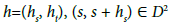 and
and i.e.
i.e.
 (1)
(1)
These two equivalent tools useful to characterize the correlation structure of a second order stationary STRF must be admissible; this aspect represents a key issue in modeling a covariance function or variogram [4]. By taking into account that covariance function and variogram are alternative measures of spatial correlation, in the following, geostatistical analysis will be based only on the use of variogram. As specified hereafter, it is also worth introducing the spatial and temporal marginal variograms, γST (hs, 0) and γST (0, ht), respectively.
In a space-time analysis, optimal prediction of Z at an unobserved point (s, t), with the associated prediction accuracy, is commonly of interest and is obtained through a linear combination of the observations. The linear combination that minimizes the mean squared prediction error is called the kriging predictor of Z(s, t). The weights used in the linear combination depend on the geometry of the sample points and on the space-time admissible model fitted to the estimated variogram surface. Given the observed values
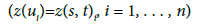
The problem is to predict Z(u)=Z(s, t) at the unsampled spacetime location u=(s, t) using the following linear predictor
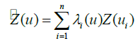 (2)
(2)
This last predictor performs interpolation and extrapolation in space and time. The weights λi, i = 1, . . . , n can be obtained by requiring that (2) is unbiased and the mean squared prediction error is minimized. Hence, the following linear system, often called ordinary kriging system, is obtained:
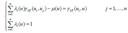 (3)
(3)
where γST represents the space-time semivariogram of Y and μ is a Lagrange multiplier.
Note that system (3) to be solved requires the knowledge of a space-time variogram model; thus, estimating and modeling the variogram are crucial steps of structural analysis. Structural analysis begins with estimating the space-time variogram of the residual random field Y.
Given the set A of data locations in space-time

the space-time variogram can be estimated through the sample space-time variogram  as follows
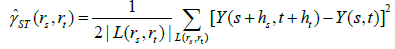 (4)
(4)
where  is the cardinality of .the set

and  are respectively, the specified tolerance regions around rs and rt. It is important to highlight that no space-time metric is defined. Indeed, the pairs of points separated by (hs, ht) are detected by computing, separately, the purely spatial and temporal distances; thus, the pairs of realizations, y(s, t) and y(s+hs, t+ht) correspond to points that are simultaneously separated by hs, in space domain, and ht, in time domain.
The second step of the structural analysis is related to the fitting process of a theoretical admissible model to the sample space-time variogram. Nowadays, various classes of space-time variogram functions are available; however the generalized product-sum model by De Iaco et al. [46] is largely used in practice in different areas, ranging from environmental sciences to medicine, from ecology to hydrology [47-51]; its efficiency and flexibility, compared with other classes of correlation functions, have been pointed out through a comparative study in De Iaco et al. [20]
The generalized product-sum model has its power in the flexibility of the fitting process, which uses the sample marginal and only one parameter that depends on the global sill. Thus, this model has been proposed for modeling the spatio-temporal correlation structure under study.
The generalized product-sum model is defined as follows:
 (5)
(5)
where γST (hs, 0) and ST (0, ht) are valid spatial and temporal bounded variograms and
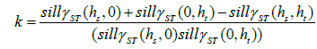 (6)
(6)
Basic theoretical results are given in De Iaco et al. [46], moreover recently it was shown that strict conditionally negative definiteness of both marginals is a necessary as well as a sufficient condition for the generalized product-sum (5) to be strictly conditionally negative definite [52].
After modeling the spatial and temporal marginal variograms and the corresponding sills, the parameter k is chosen, so that the sufficient condition of admissibility for γST (hs, ht) is properly satisfied, namely:
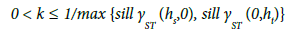 (7)
(7)
Exploratory analysis
In the following, the PM10 average concentrations have been analyzed and discussed; however an extension to other variables included in the available environmental data set is straight forward. In particular, the explored spatio-temporal data regard the daily concentrations of PM10 observed for the month of November 2009 at 28 monitoring stations located in the Salento region (i.e, the three provinces of Lecce, Brindisi and Taranto).
After geo-referencing the environmental network, the location map of the monitoring stations of PM10, which are active in 2009 in the Salento region, has been obtained (Figure 5). Note that the size of the symbols is proportional to the intensity of the value measured in corresponding monitoring stations.

Figure 5: Location map concerning the monitoring stations of PM10, active in 2009 in the Salento region.
It is worth pointing out that the highest concentrations of PM10 have been found in some stations located in Lecce and Taranto.
Regarding to the temporal structure, the time series of the PM10 daily average for the month of November 2009, in each location, are shown in Figure 6. The highest peak of PM10 concentrations has been detected in the province of Brindisi; however, the threshold value (50 μg/m3) has been exceeded in the whole region: such as in the stations called Campi Salentina and Guagnano (identified with the code 205 and 209, respectively) in Lecce province or in the station, called Machiavelli (code 302), in Taranto province.

Figure 6: The time series regarding the average daily value measured of PM10 concentrations (measured in μg/m3), for the month of November 2009, in each province belonging to the Salento Region.
Spatio-temporal analysis
The spatio-temporal analysis of the daily average concentrations of PM10 has been developed by means of:
• The structural analysis, which covers the estimation of the space-time variogram and the fitting procedure of an appropriate model such as the generalized product-sum model [46,52,53];
• The application of spatio-temporal kriging for the week from the 1st to the 8th of December 2009.
To this end, some GSLIB routines [7] suitably modified by De Iaco et al. [22] have been used. Please refer to the literature for further details regarding the geostatistical space-time analysis in the environmental field [22,51,54-61]. The empirical marginal variograms for PM10 and the corresponding models are illustrated in Figure 7, while the analytical expressions are given below:
 (8)
(8)
 (9)
(9)

Figure 7: The empirical marginal variograms and the corresponding models for PM10: A) temporal, B) spatial.
where Gauss (.) and Exp (.) stand for the Gaussian and exponential models, respectively [62]. After modeling the marginals, k in (5) is the only parameter to be estimated; this parameter can be determined by using the sill values of the marginals and the global sill (the limiting value of the variogram surface), under the condition (7).
Thus, the spatial and temporal sill values have been obtained from the models (8) and (9), while the global sill value, equal to 320, has been evaluated graphically by analyzing the sample spatio-temporal variogram surface (Figure 8).

Figure 8: The empirical spatio-temporal variogram surface for PM10.
On the basis of the sill values previously estimated, the estimate of k is given below:
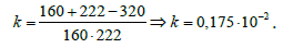 (10)
(10)
At the end, predictions for the PM10 daily average concentrations, from the 1st to the 8th of December 2009 at each monitoring station, have been produced through ordinary kriging.
Web-GIS Implementation
The Web-GIS is a geographic information system characterized by the following features: online accessibility of geographic data and data files, updated data in real-time and selection of geographic information by themes. Indeed, the users can simultaneously access to the latest data on multiple servers located in different locations; thus this greatly expands GIS data management capabilities [63]. In this section, a description of the new Web-GIS is provided. This Web-GIS includes the tabular and graphical information stored in the already presented GIS and the main results obtained from the geostatistical analysis of the measured pollutants. It should be noted that the realization of this tool, hereinafter called Geo Web-GIS, requires the use of a specific software for the online data access. With regard to this aspect, it worth pointing out that the Open Source Map Server software has been used [64], since today it represents one of the best servers for online publication of geographical information as well as for Web-GIS functions implementation. In particular, the interface for the implemented Geo Web-GIS has been obtained by using the p. mapper 4.1.1 software which is able to develop interactive interfaces, through the features available in modern browsers.
Main characteristics
The Geo Web-GIS represents a prototype for the provinces of Brindisi, Lecce and Taranto and implements vector data in ESRI shape file, raster and grid. Taking into account that this Web-GIS aims to support environmental monitoring issues, several geographic data have been included, such as: the administrative features, the monitoring network, and the raster data of the territory under study.
In the proposed Geo Web-GIS, alphanumeric information associated with geographic features of interest can be displayed through the use of appropriate tables; the connection to other web pages or database can be implemented through suitable hyperlinks functions.
By exploiting the Geo Web-GIS homepage (Figure 9), the user can have detailed information about, for example, the air quality monitoring stations located in the area of interest; moreover one can also access to the section titled “Geostatistical analysis,” where the descriptive analysis of the concentrations of the main pollutants detected by ARPA Puglia network, the spatial distribution of the air pollutants and forecasts are available. It is not excluded the possibility to implement also the results of multivariate geostatistical analysis [47,65].

Figure 9: Homepage of the Geo Web-GIS for the Salento region.
Through specific queries on thematic maps, one can display, the data stored in tabular form. Interactive navigation of maps is made possible by the functionality implemented in the Geo Web-GIS, such as the use of zooming/panning available by selecting the object on the map. In addition, one can make a print layout of a thematic map of particular interest, or save a data file or an executable file. The Geo Web-GIS application also displays information about the parameters related to the geographical reference system, the unit of measurement of the coordinates and the reference system used (that is ED1950 UTM Zone 32N). In order to ensure the interoperability (i.e. exchange and/or sharing) of geographic data, it has been relevant to build a Geo Web-GIS according with the specifications of the services defined by the Open Geospatial Consortium (OGC). In fact, by using the features implemented in the Geo Web-GIS, the users can also integrate data located on different servers as well as data of different formats. This is possible by recalling the Web Map Service (WMS) given by the OGC that avoids duplication of data and, at the same time, provides updated geographical data which are certified by shared Standards. Moreover, in addition to WMS, even the Web Feature Service (WFS) and the Web Coverage Service (WCS) are used to encapsulate the standard spatial information Web Service as a Web component [66]. The service is based on the Web Service approach to achieve the integration of the entire system. For example, it is worth highlighting that by using the WMS service of Geographic Information System of the Apuglia region, the thematic map of land use can be easily implemented (Figure 10). The OGC standard protocol for Web-Based GIS allows, therefore, dynamic visualization of geo-referenced thematic maps, integration and interoperability of geographic information [67-76].

Figure 10: Thematic map on land use in the Salento region, obtained by connecting WMS.
With reference to the “Administrative data”, one can activate various layers and display, for example, the boundaries of provinces, municipalities, and its urban centers of the study area, as shown in Figure 11. The “search for” function, in top right of the framework p.mapper 4.1.1, has been also used to query the database associated with the layer “Urban Centre” and to display, by using both the tabular form and the thematic map, all urban centers classified by province. In addition, other layers of information related to environmental monitoring stations can be overlaid. For example, the layer, called “Stations of PM10”, allows the users to locate the 28 monitoring stations for PM10, classified by type of station, in the Salento region as well as to perform queries on the same database, as illustrated in Figure 12. In particular, by using the query function, a table is shown up on the “Stations of PM10” layer, with information associated with, for example, station type, type of area, detected pollutants, province and link to the photographic details of the monitoring station.

Figure 11: Thematic map on the administrative boundaries of the Salento region and result of a query on the layer “Urban Centre” through the “search for” mode.

Figure 12: Result of a query on monitoring stations in the Salento region.
Implemented geostatistical results
In the following, after presenting the thematic maps produced in Geo Web-GIS, the main results of the space-time geostatistical analysis are introduced. Moreover, the level curves of the annual mean concentrations of PM10 (year 2009) have been also included in the Geo Web-GIS. In Figure 13, this geo-referenced contours map and the “Stations of PM10” layer have been overlapped. It should be noted that, in the province of Lecce, the highest concentration of PM10 is found near to peripheral stations, on the other hand, in the province of Taranto, the highest concentration of PM10 has been recorded near to industrial stations. Besides this graphical representation, one can explore more details on the data stored through the use of descriptive analysis.

Figure 13: Thematic map with overlay of the contour map for PM10 yearly mean concentrations and the location map of the monitoring stations for PM10 classified by type of station.
In the “Main results of Geostatistics” section, there is a subsection devoted to the spatio-temporal analysis, from which the user can get contour maps, in .avi format, of the monthly average concentration of PM10 for the year 2009. Through the interactive button “Weather”, the implemented video of space-time forecasts for the daily average concentrations of PM10 can be viewed. It is worth clarifying that these forecast maps have been obtained by using daily average concentrations of November 2009 and they are related to the first eight days of December. Obviously, predictions implemented in this section represent just an example, but they would require continuous updating in order to have videos and maps for at least one week forward with respect to the available observed data. In addition, the Geo Web-GIS system allows the users to select one or more forecast maps related to the level of pollution by PM10 over the area of interest (Figure 13) and to include significant layers, such as the location map of the monitoring stations (Figure 14). In particular, within the same section, the users can activate the layer “Estimates and Errors” and get the estimates of daily average concentrations of PM10 for each monitoring station, by using the “identify” tool in the navigation bar (Figure 14).

Figure 14: Selection of PM10 forecast results and their representation together with the location map of the monitoring stations for PM10.
Finally, through the Geo Web-GIS, the users can activate the control instrument, called Query Editor, which allows the users to submit a request of geographic information which is not defined a priori in the “search for” function. Figure 14 shows the thematic map and the table generated automatically by a new Query Editor command. This command allows the PM10 monitoring stations to be selected according to the station type (“Traffic”, “Industrial”, “Peripheral”) and the number of exceeding days (i.e. days where concentrations of PM10 are greater than the legal threshold corresponding to 50 μg/m3) that have been registered. In Figure 15 the results obtained by selecting
a) stations of “Traffic” type and b) a number of exceeding days at least equal to 10 (during the year 2009), have been illustrated.

Figure 15: Results of using the Query Editor Control tool in the Geo Web-GIS.
In conclusion, note that the Geo Web-GIS provides the opportunity to save a data file or a thematic map in .jpg format.
Integration of a Web-GIS Project in Google Earth
Google Earth is a Web Mapping for which two licenses are available: a free version, called Google Earth and a commercial version, called Google Earth Pro. In particular, a Web Mapping is used to generate maps with different geographic features referred to a given a coordinate system and a specific graphic format for raster and vector data. Many images generated in Google Earth derive from NASA and Digital Globe. Furthermore, Google Earth, as a client, allows the users to view the earth’s surface in 3D with different types of scales.
In this paper two ways of accessing to Google Earth information and of integrating data in a GIS project into a Google Earth environment have been presented. In the first case it is possible to use the Map Server Project; in the second case the application of Google Earth can be considered.
In particular, as shown in Figure 16, there is a specific tool, from the top left corner of the P mapper, which allows the users to access to the satellite picture of Salento region by Google Earth.

Figure 16: From Geo Web-GIS to Google Earth.
Thus, the Web-GIS gives to a potentially unlimited number of users the possibility to access and visualize geospatial information not provided in the Geo Web-GIS. Hence, the geostatistical predictions, for the concentrations of PM10 and the auxiliary information regarding the monitoring network can be easily integrated inside a geo browser, such as Google Earth. In the following the steps which allow the integration of geographic data stored in a GIS project inside Google Earth have been described:
• Converting the data used in GIS project, from UTM ED50 metric system to WGS84 cartographic system, that is the cartographic system used in Google Earth;
• Organizing and saving with appropriate tools, such as ArcGIS and other Open Source software, geographic data to allow the access to this geospatial information through an interface such as Google Earth.
It is important to underline, that the Google Earth applications use the specifications of KML (Keyhole Mark-up Language), that is a XML language, defined by OGC, useful to view the geographical information.
For instance, in Figure 17 the prediction map of the 3rd of December 2009 for PM10 concentrations is shown. This prediction map has been integrated with different layers available from the realized GIS project and belongs to a KML file, accessible through the Web. This KML file allows a great number of users to display and manage geographic information over the Salento region, as well as, to display the main results of the spatio-temporal analysis carried out for the PM10 pollutant. The potentiality of the cartography on the internet and the possibility for each user to use it for specific needs, stimulate further developments of Web applications.

Figure 17: Implemented maps in Google Earth for the variable PM10.
Conclusion
In this paper, after introducing the usefulness of geostatistical tools supported by a GIS, the results of the spatio-temporal geostatistical analysis on an environmental data set related to the Salento region have been discussed and the construction of a Web-GIS for the same environmental data has been presented. In particular, an ad-hoc Web-GIS, called Geo Web-GIS, has been proposed. The prediction maps of daily concentrations of PM10 obtained by using ordinary spatio-temporal kriging, based on the product-sum variogram model, have been stored into the Geo Web-GIS, together with several information about the monitoring stations (such as administrative characteristics, demographic data and municipal boundaries).
The proposed Geo Web-GIS strengthens the consciousness about benefits from the integration between GIS and advanced geostatistical techniques in order to support the management of a sustainable development.
Acknowledgment
The authors are grateful to the Editor and the reviewers, whose comments contribute to improve the present version of the paper.
References
- Matheron G (1963) Principles of Geostatistics. Econ Geology 58: 1246-1266.
- Journel AG, Huijbreghts CHJ (1984) Mining Geostatistics. Academic Press, London.
- Isaaks EH, Srivastava RM (1989) An Introduction to Applied Geostatistics. Oxford University Press, New York, USA.
- Christakos G (2013) Random Field Models in Earth Sciences. Elsevier, USA.
- Goovaerts P (1997) Geostatistics for natural resources evaluation. Oxford University Press, New York, USA.
- Kitanidis PK (1997) Introduction to Geostatistics: Applications in Hydrogeology. Cambridge, Cambridge University Press, USA.
- Deutsch CV, Journel AG (1998) GSLIB: Geostatistical Software Library and User’s Guide. Applied Geostatistics Series, Oxford University Press, USA.
- Remy N, Boucher A, Wu J (2009) Applied Geostatistics with SGeMS: A User’s Guide. Cambridge University Press, New York, USA.
- Geovariances (2015) Isatis software, Geovariances, Avon, France.
- R Core Team (2017) R: A Language and Environment for Statistical Computing. R Foundation for Statistical Computing, Vienna, Austria.
- Pebesma EJ, Wesseling CG (1998) Gstat: a program for geostatistical modelling, prediction and simulation. Computers & Geosciences 24: 17-31.
- Pebesma EJ (2004) Multivariable geostatistics in S: the gstat package. Computers & Geosciences 30: 683-691.
- Pebesma EJ, Bivand RS (2005) Classes and Methods for Spatial Data in R. R News 5: 9-13.
- Ribeiro PJ, Diggle PJ (2001) GeoR: A Package for Geostatistical Analysis. R News 1: 15-18.
- Diggle PJ, Ribeiro PJ (2007) Model Based Geostatistics. Springer-Verlag, New York, USA.
- Melo C, Santacruz A, Melo O (2015) Geospt: An R Package for Spatial Statistics. R package version 1.0-2
- Schlather M, Malinowski A, Menck PJ, Oesting M, Strokorb K (2015) Analysis, Simulation and Prediction of Multivariate Random Fields with Package RandomFields. Journal of Statistical Software 63: 1-25.
- Renard D, Desassis N, Beucher H, Ors F, Laporte F (2014) RGeostats: The Geostatistical Package. Mines Paris Tech. Centre for Geosciences, France.
- Laurent T, Ruiz-Gazen A, Thomas-Agnan C (2012) GeoXp: An R Package for Exploratory Spatial Data Analysis. Journal of Statistical Software 47: 1-23.
- De Iaco S (2010) Space–time correlation analysis: a comparative study. Journal of Applied Statistics 37: 1027-1041.
- Pebesma EJ (2012) space time: Spatio-Temporal Data in R. Journal of Statistical Software 51: 1-30.
- De Iaco S, Maggio S, Palma M, Posa D (2012) Towards an automatic procedure for modeling multivariate space–time data. Computers & geosciences 41: 1-1.
- Gabriel E, Rowlingson B, Diggle PJ (2013) stpp: An R Package for Plotting, Simulating and Analysing Spatio-Temporal Point Patterns. J Stat Softw 53: 1-29.
- Burrough PA, McDonnell RA, Lloyd CD (2015) Principles of geographical information systems. Oxford University Press, USA.
- Burrough PA (2001) GIS and geostatistics: Essential partners for spatial analysis. Environmental and ecological statistics 8: 361-377.
- Heuvelink GBM (1998) Error Propagation in Environmental Modeling with GIS. Taylor and Francis, London, UK.
- De Paz JM, Albert C, Visconti F, Jimenez MG, Ingelmo F, et al. (2015) A new methodology to assess the maximum irrigation rates at catchment scale using Geostatistics and GIS. Precision Agric 16: 505-531.
- Hsiao DW, Trappey AJ, Ma L, Ho PS (2009) An integrated platform of collaborative project management and silicon intellectual property management for IC design industry. Information Sciences 179: 2576-2590.
- Li J, Huai J, Hu C, Zhu Y (2010) A secure collaboration service for dynamic virtual organizations. Information Sciences 180: 3086-3107.
- Richards D (2009) A social software/Web 2.0 approach to collaborative knowledge engineering. Information Sciences 179: 2515-2523.
- Zhu D, Li Y, Shi J, Xu Y, Shen W (2009) A service-oriented city portal framework and collaborative development platform. Information sciences 179: 2606-2617.
- Zhang J, Gong J, Lin H, Wang G, Huang J, et al. (2007) Design and development of distributed virtual geographic environment system based on web services. Information Sciences 177: 3968-3980.
- Xu B, Lin H, Chiu L, Hu Y, Zhu J, et al. (2011) Collaborative virtual geographic environments: a case study of air pollution simulation. Information Sciences 181: 2231-2246.
- Goodchild M, Haining R, Wise S (1992) Integrating GIS and spatial data analysis: problems and possibilities. International journal of geographical information systems 6: 407-423.
- Anselin L (2000) Computing environments for spatial data analysis. Journal of Geographical Systems 2: 201-220.
- Bivand R, Gebhardt A (2000) Implementing functions for spatial statistical analysis using the language. Journal of Geographical Systems 2: 307-317.
- Boots B (2000) Using GIS to promote spatial analysis. Journal of Geographical Systems 2: 17-21.
- Wise S, Haining R, Ma J (2001) Providing spatial statistical data analysis functionality for the GIS user: the SAGE project. International Journal of Geographical Information Science 15: 239-254.
- Henshaw SL, Curriero FC, Shields TM, Glass GE, Strickland PT, et al. (2004) Geostatistics and GIS: Tools for Characterizing Environmental Contamination. Journal of Medical Systems 28: 335-348.
- Pebesma EJ (2006) The Role of External Variables and GIS Databases in Geostatistical Analysis. Transactions in GIS 10: 615-632.
- Peterson EE, Scott UN (2006) Predicting Water Quality Impaired Stream Segments Using Landscape-Scale Data And A Regional Geostatistical Model: A Case Study In Maryland. Environmental Monitoring and Assessment 121: 615-638.
- Shit PK, Bhunia GS, Mait R (2016) Spatial analysis of soil properties using GIS based geostatistics models. Information Sciences Model. Earth Syst Environ 2: 107-112.
- De Iaco S, Posa D (2012) Predicting spatio-temporal random fields: some computational aspects. Computers & geosciences 41: 12-24.
- Wesselung CG, Karssenberg DJ, Burrough PA, Deursen W (1996) Integrating dynamic environmental models in GIS: the development of a Dynamic Modelling language. Transactions in GIS 1: 40-48.
- Banerjee J, Chou HT, Garza JF, Kim W, Woelk D, et al. (1987) Data model issues for object-oriented applications. ACM Transactions on Information Systems (TOIS) 5: 3-26.
- De Iaco S, Myers DE, Posa D (2001) Space–time analysis using a general product–sum model. Statistics & Probability Letters 52: 21-28.
- De Iaco S, Myers DE, Posa D (2002) Space–time variograms and a functional form for total air pollution measurements. Computational Statistics & Data Analysis 41: 311-328.
- Fernández-Casal R, González-Manteiga W, Febrero-Bande M (2003) Flexible spatio-temporal stationary variogram models. Statistics and Computing 13: 127-136.
- Gething PW, Noor AM, Gikandi PW, Ogara EA, Hay SI, et al. (2006) Improving imperfect data from health management information systems in Africa using space–time geostatistics. PLoS Medicine 3: e271.
- Skøien JO, Blöschl G (2006) Catchments as space-time filters? A joint spatio-temporal geostatistical analysis of runoff and precipitation. Hydrology and Earth System Sciences Discussions 3: 941-985.
- Spadavecchia L, Williams M (2009) Can spatio-temporal geostatistical methods improve high resolution regionalisation of meteorological variables?. Agricultural and Forest Meteorology 149: 1105-1117.
- De Iaco S, Myers DE, Posa D (2011b) Strict positive definiteness of a product of covariance functions. Communications in Statistics-Theory and Methods 40: 4400-4408.
- De Iaco S, Myers DE, Posa D (2011a) On strict positive definiteness of product and product–sum covariance models. Journal of Statistical Planning and Inference 141: 1132-1140.
- Kolovos A, Christakos G, Hristopulos DT, Serre ML (2004) Methods for generating non-separable spatiotemporal covariance models with potential environmental applications. Advances in Water Resources 27: 815-830.
- Cocchi D, Greco F, Trivisano C (2007) Hierarchical space-time modelling of PM10 pollution. Atmospheric environment 41: 532-542.
- Calder CA (2008) A dynamic process convolution approach to modeling ambient particulate matter concentrations. Environmetrics 19: 39-48.
- Paciorek CJ, Yanosky JD, Puett RC, Laden F, Suh HH (2009) Practical large-scale spatio-temporal modeling of particulate matter concentrations. The Annals of Applied Statistics 1: 370-397.
- Cressie N, Wikle CK (2015) Statistics for spatio-temporal data. John Wiley & Sons, New Jersey, USA.
- Fasso A, Finazzi F (2011) Maximum likelihood estimation of the dynamic coregionalization model with heterotopic data. Environmetrics 22: 735-748.
- De Iaco S, Myers DE, Palma M, Posa D (2010) FORTRAN programs for space–time multivariate modeling and prediction. Computers & Geosciences 36: 636-646.
- Bevilacqua M, Gaetan C, Mateu J, Porcu E (2012) Estimating space and space-time covariance functions for large data sets: a weighted composite likelihood approach. Journal of the American Statistical Association 107: 268-280.
- Chiles J, Delfiner P (2012) Geostatistics - Modeling spatial uncertainty. Wiley, New York, USA.
- Tan J, Li SH, Zeng JY, Wu XJ (2015) Antioxidant and hepatoprotective activities of total flavonoids of indocalamus latifolius. Bangladesh Journal of Pharmacology 10: 779-789.
- Kropla B (2005) Beginning MapServer: Open Source GIS development. Apress, New York, USA.
- De Iaco S (2011) A new space–time multivariate approach for environmental data analysis. Journal of Applied Statistics 38: 2471-2483.
- Cui HR, Liu FX, Armentani E (2016) Analysis and assessment of the value of carbon assets based on montecarlo simulation. Journal of Mechanical Engineering Research and Developments 39: 555-564.
- Austenfeld M, Beyschlag W (2012) A Graphical User Interface for R in a Rich Client Platform for Ecological Modeling. Journal of Statistical Software 49: 11-19.
- Banerjee J, Chou HT, Garza JF, Kim W, Woelk D, et al. (1987) Data model issues for object-oriented applications. ACM Transactions on Information Systems (TOIS) 5: 3-26.
- Cressie N (2015) Statistics for spatial data. John Wiley & Sons, USA.
- Date CJ (1983) An introduction to database systems. Addison- Wesley, Boston, Massachusetts, USA.
- De Iaco S, Maggio M, Palma M (2017) Radon Predictions with Geographical Information System covariates: From Spatial Sampling to Modeling. Geographical Analysis 49: 215-235.
- De Iaco S, Posa D, Myers DE (2013) Characteristics of some classes of space–time covariance functions. Journal of Statistical Planning and Inference 143: 2002-2015.
- Statios LLC (2001) WinGSLIB: Geostatistical Software Library, version 1.4.
- Stephen W (2014) GIS foundamentals . CRC Press, Taylor& Francis Group, NewYork, USA.
- Waller LA, Gotway CA (2004) Applied spatial statistics for public health data. John Wiley & Sons, USA.
- Zhu J, Gong J, Liu W, Song T, Zhang J (2007) A collaborative virtual geographic environment based on P2P and Grid technologies. Information Sciences 177: 4621-4633.