Spanish
  Chinese
  Russian
  German
  French
  Japanese
  Portuguese
  Hindi
Hindi Research Article, Geoinfor Geostat An Overview Vol: 6 Issue: 3
Polynomial Separation and Gravity Data Modeling with Hyperbolic Density Contrast: Case of Two Profiles along the Mamfe Sedimentary Basin (Cameroon)
Nguimbous-Kouoh JJ1*, Takam-Takougang EM2, Ndougsa-Mbarga T3 and Manguelle-Dicoum E4
1Department of Mineral, Petroleum, Gas and Water Resources Exploration, Faculty of Mines and Petroleum Industries, University of Maroua, Maroua, Cameroon
2Department of Exploration Geophysics, KUST-The Petroleum Institute, Abu Dhabi, Saudi Arabia
3Department of Physics, Advanced Teacher’s Training College, University of Yaounde, Yaounde, Cameroon
4Department of Physics, Faculty of Science, University of Yaounde, PO Box 6052 Yaounde, Cameroon
*Corresponding Author : Nguimbous-Kouoh JJ
Department of Mineral, Petroleum, Gas and Water Resources Exploration, Faculty of Mines and Petroleum Industries, University of Maroua, Maroua, Cameroon
Tel: (+237) 699674 060
E-mail: nguimbouskouoh@yahoo.fr
Received: April 06, 2018 Accepted: May 23, 2018 Published: May 30, 2018
Citation: Nguimbous-Kouoh JJ, Takam-Takougang EM, Ndougsa-Mbarga T, Manguelle-Dicoum E (2018) Polynomial Separation and Gravity Data Modeling with Hyperbolic Density Contrast: Case of Two Profiles along the Mamfe Sedimentary Basin (Cameroon). Geoinfor Geostat: An Overview 6:2. doi: 10.4172/2327-4581.1000187
Abstract
The primary objective of a gravity survey over a sedimentary basin is to delineate the shape of the basin. To fulfill this objective, information is needed about the densities within the sedimentary section. Densities of sedimentary rocks increase with depth (mainly due to compaction), approaching that of the basement in deep
basins. Sedimentary basins are generally associated with low gravity values due to lower density of the sedimentary infill. Further, gravity modeling of a basin requires the use of expressions with hyperbolic density contrast concerning the anomaly produced by the model. The variation of the density of sediments with depth
can be represented by a hyperbolic function. In this study, a thirdorder polynomial filtering of Bouguer gravity data from the Mamfe sedimentary basin was performed. The regional and residual third order anomaly maps were fitted for interpretation. Two profiles were plotted above two negative anomalies observed on the basin.
Using the gravity data of both profiles, a workflow was developed to determine the shape and depth of an interface underlying sediments whose density contrast decreases hyperbolically with depth. The approximate depth of the interface at each gravity station was calculated using the gravity formula of an infinite slab with a hyperbolic density contrast. Based on the depth values, the sediment/basement interface were replaced by a sided polygon. The estimated depths of the sediment/basement interfaces along the two profiles above the Mamfe sedimentary basin gave 1900 and 5073 m, respectively
Keywords: Gravity anomalies; Hyperbolic density contrast; Mamfe basin
Introduction
Several studies have been carried out on the Mamfe sedimentary basin in various disciplines [1-23]. The purpose of this work is to provide additional structural information of the basin, using gravity data.
In general the density of sedimentary rocks in a basin increases with depth, the contrast in densities of the sediments and the basement thus decreases. Gravity modeling of such sedimentary basins requires the use of anomaly expressions of models with variable density contrast. While interpreting gravity anomalies of the San Jacinto Graben (California), Cordell [24] assumed an exponential variation for the sediment density. Gravity anomalies of even simple geometric bodies cannot be derived in a closed form if the variation in density contrast is exponential. As such Cordell [24] used a recursive algorithm in the interpretation of the San Jacinto Graben gravity profile. Murthy et al. [25] and Agarwal [26] considered the case of linear increase in density with depth in gravity modeling of sedimentary basins. Rao [27] used a quadratic density function for approximating the variation in density of sediments. This quadratic representation amounts to using the first three terms of the infinite series expansion of the exponential function. It may fail to represent the variation in density contrast beyond the depth of approximation. Litinsky [28] introduced a hyperbolic density depth function and found that in the case of the San Jacinto Graben this function could provide a better fit for the density at depths than did the exponential function. When the density contrast is assumed to vary with depth according to the hyperbolic function, closed form of anomaly expressions of models can be derived and simple modeling or inversion schemes developed. However, Litinsky [28] used a simple formula of gravity anomaly of an infinite slab with effective hyperbolic density contrast for calculating the thickness of sediments at different gravity stations. It is observed that the use of this formula generates errors.
In this paper, we used the closed-form expression for the gravity anomaly of a two-dimensional arbitrary shaped body with a hyperbolic density contrast derived by Rao et al. [29]; we developed an algorithm (Appendix) to model and find the basement of sediments at various gravity stations, using two profiles in the Mamfe sedimentary basin.
Geology of the Study Area
The Mamfe sedimentary basin is an intracratonique rift basin formed in response to the dislocation of the Gondwana supercontinent and following the separation of South American and African plates (Figure 1). The basin is a small extension of the Benue sedimentary basin (Figure 1). The basin is favorable to the exploration and exploitation of salt springs, minerals, precious stones and hydrocarbons. It has an area of approximately 2400 km2 and is located between latitudes 5°30’ N and 6°00’ N and longitudes 8°40’ E and 9°50’ E (Figure 1). It has the form of a plain with an average altitude that varies between 90 and 300 m above the sea level. Its average crustal thickness is between 33 and 40 km and the coat is at a depth of about 57 km [1-23].

Figure 1: Geologic Map of the Mamfe Sedimentary Basin by Ajonina et al. [22].
Figure 1 shows the available geological map of the basin. Some geological details were extrapolated or removed. The geological map is preliminary and has jointly been updated following several studies. The geomorphology of the area is characterized by a succession of horst and grabens. Overall, the Mamfe sedimentary basin has a NW-SE structural trend with a length of 130 km and a width of approximately 60 km. It is bordered by faults, lineaments and rivers such as Manyu, Munaya and extends from Cameroon to Nigeria [1-23].
Lithologically, the basin is formed by thick Cretaceous age sediments whose thickness can vary according to the study site. It rests on granite-gneissic bedrock of Precambrian age. The order of the geological formations, from bottom to top, has a succession of granite, shale, sandstone, clays and laterite. The lamination forms a typical sigmoid syncline structure which are oriented E-W and plunge axes of 10° to about 20° W.
The tectonic history of the basin highlights the structures and synto post-sedimentary which has two main phases:
• An expansion phase characterized by sedimentation
• A compression phase during which sedimentation ended and the basin was closed.
The compression phase resulted in the creation of anticlinal and synclinal structures, horst and grabens deeding NW-SE. The phase of sedimentation and extension resulted in the creation of faults and syn-sedimentary folds [1-23].
Data Acquisition and Processing
The map presents gravity data collected over the Mamfe sedimentary basin. It was taken from the archives of the Cameroon gravity database that manages IRD (Research Institute for Development) (Figure 2). The Lacoste-Romberg gravimeter (1975- 1976) and its accessories were used to collect the data. Barometric leveling was determined using a Wallace-Tiernan altimeter. The gravity network of the IRD established in Douala served as a reference base for measurements.

Figure 2: Map of collecting gravity data over Mamfe sedimentary basin.
The Bouguer anomaly at each station was calculated by the expression Poudjom et al. [30]: B=G-(G0-Cz-T) where:
• G is the observed gravity field value and its expression is: G=Gr+ΔG with Gr the gravity field value at the station adopted as reference and ΔG the measurement of the gravity field difference between the reference station and a given station. The reference value was chosen in the Martin network (1954) and attached to the fundamental point of the Paris Observatory.
• G0 :the theoretical value of the gravity field on the reference ellipsoid has been defined in the IGSN71 reference system whose formula is:
• G0=978031.8(1+0.053024sinÕ2)-0.0000022sin2 Õ2
• The error on the latitude of a station was taken between 0.2 mgal (Õ=3°) and 0.5 mgal.
• CZ: Bouguer correction. It represents the sum of the free air correction C1 (mgal) = 0.3086Z and the plateau correction C2 (mgal)=-0.0419dZ where d is the density of the land and Z the altitude of the station expressed in meters. For the homogeneity reasons we have adopted the crust density d = 2.67 for all the stations from where Cz (mgal)=0.1967Z. The inaccuracy of the barometric leveling leads to an error on Cz generally less than 1 mgal but which can reach 2 or 3 mgal equals in unfavorable cases.
• T: relief correction. It takes into account the relief around the station. The value of the anomaly at each point is tainted by a maximum error of 5 mgal under the worst conditions, in most cases the error remained below 3 mgal.
Methods
The polynomial separation method
The polynomial separation method was used to produce the third degree regional and residual maps. The algorithm by Gupta [31] and Murthy et al. [32], was used to adjust the polynomial surfaces to the Bouguer anomaly map. This method is based on the analytical least square method and the polynomial decomposition series.
The least-square method is used to compute the mathematical surface which gave the best fits to the gravity field within specific limits [31-33]. This surface is considered to be the regional gravity anomaly. The residual is obtained by subtracting the regional field from the observed gravity field. In practice, the regional surface is considered as a two-dimensional polynomial. The order of this polynomial depends on the complexity of the geology in the study area. The third-order polynomial surfaces of the regional anomaly obtained in this work is presented and the corresponding residual anomaly.
Mathematic formulation of the method: The Bouguer anomaly B(x, y) in the given point M(x, y) of the earth in Cartesian coordinates is governed by the relation:
B(xi, yi)= A(xi, yi)+ R(xi, yi) (1)
B(xi, yi)is the sum of the residual anomaly A(xi, yi) and the regional anomaly R(xi, yi).
The surface F(xi, yi)which is adapted to the gravity field data g(x, y) is given by the following relation [31-33]:
 (2)
(2)
Where N is the order of the polynomial, 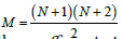 the number of terms of the polynomial, and Cm the coefficients to be determined:
The first order Polynomial is:
F(xi, yi)=C1+C2Xi+C3Yi (3)
The second order polynomial is:
 (4)
(4)
The third order polynomial is:
 (5)
(5)
We denote by εi= B(xi, yi)- F(xi, yi) the difference between the homologous points of the experimental and analytical surfaces respectively and by N0 the number of stations Pi in which the Bouguer anomaly is known. The adjustment of the surfaces which consists in making the quadratic deviation minimal is expressed by:
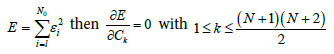 (6)
(6)
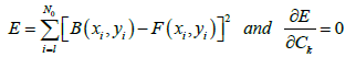
We then obtain a system of (M) equations with (M) unknowns. The unknowns are the coefficients Ck of the polynomial F(xi, yi) of order N. Once the coefficients are determined we determine the analytic regional anomaly R(xi, yi) =F(xi, yi) and the residual by:
A(xi, yi)= B(xi, yi)- F(xi, yi) (7)
The polynomial method is particularly used when the amplitude of the residual anomalies is negligible compared to the regional one. Apart from the polynomial method there are other methods such as the upward continuation method.
Modeling method
Density measurements and seismic surveys conducted in sedimentary basin Athy [34], Hedberg [35] and Maxant [36] shows that the density-depth relationship of sedimentary rocks does not obey a deterministic mathematical formulation due to the effects of stratigraphic layering, facies variations, diagenesis, tectonic history, cementation and compaction. For the analysis of gravity data over sedimentary basins, the density variation with depth can be approximated by a hyperbolic function as below [28]. The variable density contrast of sediments in a basin can be approximated by the formula (Figure 3):

Figure 3: A polygonal model simulating a sedimentary basin.
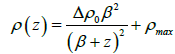
Where ρ(z) is the density contrast at depth z; Δρ0 is the density that would be observed at ground surface, ρmax is the density of the basement, and β is a constant having a unit of length and is the decrement of density contrast with increasing depth. At depth z=0 and β is the rate of variation of density contrast expressed in length units. Δρ0 and β can be determined by fitting the field data of density contrast versus depth in a least-square sense to equation:
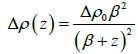 (8)
(8)
Where Δρ(z) is the density contrast at depth z; Δρ0 is the density contrast extrapolated to the ground surface, and β is the rate of variation of density contrast expressed in units of length. At any gravity station the initial depth of the interface (or thickness of the sediments) is calculated by using the infinite slab formula suitable for the case of a hyperbolic density contrast, given by Litinsky [28]:
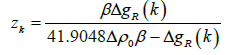 (9)
(9)
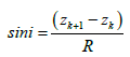
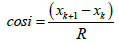
Where Δgr(k) is the residual gravity anomaly at the kth station. The sedimentary basin can now be replaced by n-sided polygon of which the verticies are defined by (xk; zk), zk is the distance of the kth station from an arbitrary reference. When the coordinates of the verticies of the polygon are known, its gravity anomaly at any point P(0) can be calculated by using the equation Rao et al. [29]:
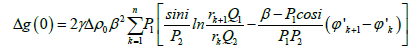 (10)
(10)
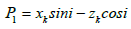
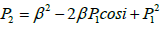


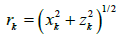

and 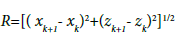 (11)
(11)
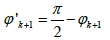
γ is the gravitational constant. The quantities xk, xk+1, zk, zk+1, φk, φk+1 and i are explained in Figure 3.
In general, the values of β and Δρ0 are unknown and can be estimated by least squares fitting to the density-depth values which are observed by borehole data in the field.
If the formation lithology, thicknesses of the formations and their density information are known from borehole data for a basin with n sedimentary layers with different thicknesses hi and different density contrasts Δρi, the weighted density constant (or average density constant) Δρ can be determined by:
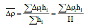
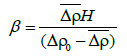
Where, H denotes the total thickness of the sediments or the depths to the basement of the basin. According to Litinsky [28], the parameter β can be estimated by two methods. If a density cross section of the basin and the values of Δρ0 and Δρ are known, β can be calculated from the equation:
The density contrast Δρ0 of surface sediments can be found from density measurements of rock samples, from borehole gravity, density logging, or from gravity data. If the values of weighted density contrast and the density contrast of the near surface sediments have been assessed, it is easy to find the parameters for the density-depth functions. On the other hand, if the depth of a sedimentary basin and the surface density are known, β can be found by using the equation:
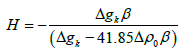
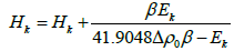
At any gravity station the initial depth of the interface, H can be calculated using the infinite slab formula for the case of a hyperbolic density constant Litinsky [28] as:
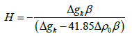
Δgk is the residual anomaly value at the kth station on the profile. The difference Ek between the residual and the calculated anomalies at any stations is attributed to the error in the depth of the interface at that station. This difference is used to correct the depth using the formula:
The modified depth values that are shallower than the ground surface are ignored and in all such cases the previous depth values are retained. This process of iteration is terminated either when the objective function R defined as the sum of the squares of differences between the observed and calculated anomalies tends to increase, falls below an allowable error or after a specified number of iterations is carried out.
Computer Program
Based on the above descriptions and mathematical expressions, we developed an algorithm named SBASIN to estimate the basement of the sedimentary layer in the basin (Appendix). This algorithm is useful to compute the gravity anomaly of a polygonal body with a hyperbolic density contrast [29,37]. The input data consist of residual gravity anomalies Δg(k) in mGals and their distances xk in km measured from the first point on the profile, the density contrast Δρ0 extrapolated to the ground surface, the hyperbolic function constant β, and N the number of anomalies. The algorithm is computed iteratively, and the output, after each iteration, consists of the basement depth in km and the gravity anomaly in mGals at each station.
Results and Interpretation
We provide a qualitative interpretation of the anomaly map derived from the polynomial separation method, and the basement/ sediment interface estimated from the hyperbolic density function using the gravity formula on an infinite slab with hyperbolic density contrast.
Interpretation of the anomaly map
Gravity anomalies, in general, are a function of horizontal variations in rock densities beneath the surface of the earth; therefore, the interpretation of gravity anomalies depends upon density contrasts. Depth-size relationships possible from geological considerations in the area involved are also necessary. The precision of the gravity survey and the amount of geological information at hand determine what type of interpretation may be made. The interpretation of gravity anomalies may be classified as qualitative or quantitative. Here, we provide a qualitative interpretation of gravity anomalies. In some instances, qualitative interpretation may be considered as diagnostic.
Interpretation of the Bouguer anomaly map: The Bouguer anomaly map reflects the steady and continuous variations of the gravity field over Mamfe Basin (Figure 4). Generally, it represents the superposition of long wavelength anomalies (regional anomalies) and short wavelength anomalies (residual anomalies) of potentially important interests depending on the application. The map shows a zone of strong gradient in the center of the basin. These indicate the occurrence of subsurface density discontinuities such as faults and boundaries of intrusive bodies. Since we want to evaluate the depth of the sediment/basement interface, we will adjust the effects of deep sources (regional anomaly) and subtract them from Bouguer anomalies to obtain (residual) surface anomalies. To separate the regional and the residual, we applied a polynomial filter.

Figure 4: Map of Bouguer anomalies in the Mamfe sedimentary basin.
Interpretation of the regional anomalies map: The regional anomaly map may represent the effect of long-wave discontinuities (Figure 5). It can also be considered as noise or as important signals if it is necessary to find the existing relations between the mantle and the earth’s crust or when it is necessary to describe the shape of the base or the lithosphere. The map shows overall regional trends affecting the basin. These trends are N-S, E-W. The different anomalies observed are either positive or negative according to the contours variation direction. Low (negative) anomalies can be associated with areas of bedrock dilation and magmatic upwelling, while high (positives) anomalies may correspond to platform or consolidation zones of basement rocks. This is probably due to a good isostatic readjustment or an unstable and complex geological context of the region.

Figure 5: Regional anomalies Map of the mamfe basin.
Interpretation of the residual anomalies map: Residual anomalies are mainly produced by heterogeneities located in the upper crust. These are often the result of mineralization or oil fields. Data from the residual gravity field were calculated after subtracting the regional trend of the Bouguer gravity field. The residual map is characterized by two negative anomalies (Figure 6). The edges of the basin are limited by several contours with strong gradient with different directions. This can be explained by the fact that the constraints that contributed to the setting up of the basin did not act in the same direction.

Figure 6: Residual anomalies Map of the mamfe basin with the two profiles.
Interpretation of the depth sediment/basement models interfaces
Two gravity anomaly profiles are interpreted using the proposed technique. The method is applied to the gravity profiles crossing the Akarem and Akagbe Grabens in the following paragraphs.
Akarem Graben, profil (NW-SE): The profile (P1) was plotted above the negative residual anomaly observed at Akarem, it is approximately oriented NW-SE. The form of the observed anomaly is a graben. The interpretation of the gravity profile on the Akarem Graben, assuming a hyperbolic density contrast for the sediments, is shown in Figure 7. The density-depth data of the graben are matched with the hyperbolic function 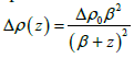 in the least squares sense. The values of Δρ0 and β are - 0.17 kg/m3 and 2850 m, respectively. The maximum depth of the interface determined by the computer program is 1900m. The objective function at the end of the 38th iteration is 3.2 and does not show any appreciable change in further iterations. The anomaly of the interpreted model was plotted against the observed one for comparison.

Figure 7: Interpretation of gravity profile over the Akarem Graben, with the density contrast varying hyperbolic with depth.
Akagbe Graben, (profil NE-SW): The profile (P2) was plotted above the negative residual anomaly observed at Akagbe, it is approximately oriented NE-SW. The form of the observed anomaly is a graben. Figure 8 show the interpretation of the gravity profile over the Akagbe Graben. A least-square fit of the data to 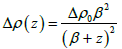 provided values of - 0.17 kg/m3 and 2850 m for Δρ0 and β respectively. The algorithm gave a maximum depth of 5073 m for the basement/ sediment interface. The best fitting solution resulted in an objective function of 3.2 at the end of the 38th interaction is show in Figure 8 against the observed anomaly.

Figure 8: Interpretation of gravity profile over the Akagbe Graben, with the density contrast varying hyperbolic with depth.
Discussion
Generally, negative anomalies are associated with basin trend patterns, while positive anomalies are associated with platform or mountain configurations. The positive effect may be due to a small crustal thickness whereas the negative effect may be due to the proximity of the magma near the surface [37].
Ndougsa-Mbarga et al. [38], using data from Fairhead et al. [5] and their regional-residual separation to the third order showed that the Mamfe basin is subdivided into two sources of negative anomalies. The data used in this work demonstrate that it is necessary to separate up to the third order to obtain a gravity field signature that fits well with the Mamfe sedimentary basin.
The area where the Mamfe Basin is located has always been considered as a graben that is associated with a negative Bouguer anomaly [5]. The data from the Bouguer map of this study confirm this result but present a basin strongly masked by the effect of the proximity of the Cameroon volcanic line deposits (CVL).
Kamguia et al. [39] studying the local geoid model in Cameroon find that this geoid undulates abnormally above the reference ellipsoid through the Mamfe basin with a value of about 27 m. They concluded that this value implies the occurrence of low density rocks in the region. The results obtained from the interpretation of the gravity field data of this study show that the zone is effectively associated with a negative Bouguer anomaly.
The sediment/basement depths estimated are quite close to those reported by Fairhead et al. [4] (600-6000m). Similar estimated depth values were also obtained by combining geomorphological data and Lansat images by Ajonina (5000 m) [40-44].
Conclusion
The interpretation of gravity field maps of the Mamfe sedimentary basin highlights some structural aspects of the area. Although the density of the data is reduced, they have been good enough to trace the pace of the shallow and deep structures of the area. They precisely adjust the results of other gravity field investigations, as well as to improve the geological and geophysical knowledge of the area. The approach used highlights the details of the regional trends and delineate the important geological structures of interest. The interpretation of the sediment/bedrock depths (1900 and 5073 m depths), which can be considered interesting for the maturation of hydrocarbon source rocks.
Acknowledgments
This study was conducted as part of research activities accomplished in the Department of Mineral, Petroleum, Gas and Water Resources Exploration of the Faculty of Mines and Petroleum Industries of the University of Maroua, north Cameroon. Special thanks to all the colleagues for their inputs and supports.
References
- Le Fur Y (1965) Mission socle-Cretace. Rapport 1964-1965 sur les indices de plomb et zinc du golfe de Mamfe. Rapport BRGM, Cameroun, Cameroon.
- Dumort JC (1968) Carte geologique de reconnaissance a lechelle 1/500000. Note explicative sur la feuille Douala-Ouest. Republique federale du Cameroun, Direction des Mines et de la Geologie du Cameroun, Cameroon.
- Paterson G, Watson A (1976) Etudes aeromagnetiques sur certaines regions de la Republique Unie du Cameroun. Rapport dinterpretation Agence Canadienne de Developpement International Toronto, Toronto, Canada.
- Fairhead JD, Okereke CS (1988) Depth to major contrast beneath the West African rift system in Nigeria and Cameroon based on the spectral analysis of gravity data. J African Earth Sci 7: 769-777.
- Fairhead JD, Okereke CS, Nnange JM (1991) Crustal structure of the Mamfe basin, West Africa, based on gravity data. Tectonophysics 186: 351-358.
- Manguelle-Dicoum E, Nouayou R, Tabod C, Kwende-Mbanwi TE (1999) Audio and Heliomagnetotelluric study of the Mamfe sedimentary basin. Tech Rep 58: 87-90.
- Kangkolo R (2002) Aeromagnetic Study of the Mamfe Basalts of South-western Cameroon. Journal of the Cameroon Academy of Sciences 2: 173-182.
- Eseme E, Agyingi CM, Foba-Tendo J (2002) Geochemistry and genesis of brine emanations from Cretaceous strata of the Mamfe Basin, Cameroon. Journal of African Earth Sciences 35: 467-476.
- Eseme E, Littke R, Agyingi CM (2006) Geochemical characterization of a Cretaceous black shale from the Mamfe Basin, Cameroon. Petroleum Geoscience 12: 69-74.
- Eseme E, Abanda PA, Agyingi CM, Foba-Tendo J, Hannigan RE (2006) Composition and applied sedimentology of salt from brines of the Mamfe Basin, Cameroon. Journal of Geochemical Exploration 91: 41-55.
- Nguimbous-Kouoh JJ (2003) Structural Interpretation of the Mamfe Sedimentary Basin of Southwestern Cameroon along the Manyu River Using Audiomagnetotellurics Survey. ISRN Geophysics 20: 52-59.
- Eyong JT (2003) Litho-Biostratigraphy of the Mamfe Cretaceous Basin, S.W. Province of Cameroon-West Africa. University of Leeds, England.
- Nouayou R (2005) The use of Aeromagnetic Data Interpretation to Characterize the Features in the Mamfe Sedimentary Basin Cameroon and a Part of the East of Nigeria. International Journal of Science and Research 6: 617-624.
- Tabod CT, TokamKamga AP, Manguelle-Dicoum E, Nouayou R, Nguiya S (2008) An Audio-Magnetotelluric Investigation of the Eastern Margin of the Mamfe Basin, Cameroon. The Abdus Salam International Centre for Theoretical Physics, Trieste, Italy.
- Ndougsa-Mbarga T, Manguelle-Dicoum E, Campos-Enriquez JO, Atangana QY (2007) Gravity anomalies, sub-surface structure and oil and gas migration in the Mamfe, Cameroon-Nigeria, sedimentary basin. Geofísica internacional 46: 129-139.
- Ajonina HN, Ajibola OA, Bassey CE (2001) The Mamfe Basin, S.E. Nigeria and S.W. Cameroon: A review of basin filling model and tectonic evolution. Journal of the Geosciences Society of Cameroon 1: 24-25.
- Ajonina HN, Betzler C, Jaramillo C (2010) Paleoclimatic significance of an Early Cretaceous fan-delta sedimentary succession in the eastern Mamfe Basin, SW Cameroon. Annual Meeting of the Africa Group of German Geoscientists, Frankfurt, Germany.
- Ajonina HN, Betzler C, Volkheimer W, Eyong JT (2008) Palynology and depositional environments of Early Cretaceous sediments in the Mamfe Basin, west Africa and their relationship to other Gondwanic regions in South America. Conference proceedings of 12th International Palynological Congress (IPC-XII) 8th International Organisation of Paleobotany Conference, Bonn, Germany.
- Ajonina HN, Betzler C, Eyong JT, Eseme E, Hell JV (2007) Stratigraphy and sedimentary evolution of the Mamfe Basin, southwest Cameroon, West Africa. 4th International Limnogeology Congress, Barcelona, Spain.
- Ajonina HN, Njilah IK, Ndjeng E, Hell JV, Bassey CE, et al. (2006) Sedimentology and reservoir potential of sandstones of the Mamfe Formation, Mamfe Basin, Southeast Nigeria and Southwest Cameroon. Science of Nature and Life 36: 117-132.
- Ajonina HN, Jaramillo C, Volkheimer W, Mejía P, Betzler C, et al. (2010) Palynostratigraphy and age of the Lower Cretaceous Mamfe Group, Mamfe Basin, SW Cameroon, eastern West Africa. In the proceedings of 8th European Palaeobotany-Palynology Conference, Budapest, Hungary.
- Ajonina HN, Betzler C, Hell JV, Eseme E, Volkheimer W, et al. (2012) Hydrocarbon potential of the Mamfe Basin, SW Cameroon. GV & Sediment Meeting 2012, Hamburg, Germany.
- Eyong JT, Wignall P, Fantong WY, Best J, Hell JV (2013) Paragenetic sequences of carbonate and sulphide minerals of the Mamfe Basin (Cameroon): Indicators of palaeo-fluids, palaeo-oxygen levels and diagenetic zones. Journal of African Earth Sciences 86: 25-44.
- Cordell L (1973) Gravity analysis using an exponential density-depth function—San Jacinto Graben, California. Geophysics 38: 684-690.
- Murthy IVR, Rao CV, Rao VN (1981) Gravity anomalies of two dimensional vertical prisms and steps of finite extent and sedimentary basins with their densities increasing linearly with depth. Bull Geophys Res 19: 73-82.
- Agarwal BN (1971) Direct gravity interpretation of sedimentary basin using digital computer—Part I. Pure and applied geophysics 86: 5-12.
- Rao DB (1986) Modelling of sedimentary basins from gravity anomalies with variable density contrast. Geophysical Journal International 84: 207-212.
- Litinsky VA (1989) Concept of effective density: Key to gravity depth determinations for sedimentary basins. Geophysics 54: 1474-1482.
- Rao CV, Chakravarthi V, Raju ML (1994) Forward modeling: Gravity anomalies of two-dimensional bodies of arbitrary shape with hyperbolic and parabolic density functions. Computers & Geosciences 20: 873-880.
- Poudjom-Djomani YH, Boukeke DB, Legeley-Padovani A, Nnange JM, Ateba B, et al. (1996) Levés gravimétriques de reconnaissance-Cameroun. Orstom, Paris.
- Gupta VK (1983) A Least Squares Approach to Depth Determination from Gravity Data. Geophysics 48: 357-360.
- Murthy IVR, Krisshnamacharyulu SKG (1990) A Fortran 77 Programme to Fit a Polynomial of Any Order to Potential Field Anomalies. Journal of Association of Exploration Geophysicists 11: 99-105.
- Nguimbous-Kouoh JJ, Ngos III S, Mbarga TN, Manguelle-Dicoum E (2017) Use of the Polynomial Separation and the Gravity Spectral Analysis to Estimate the Depth of the Northern Logone Birni Sedimentary Basin (CAMEROON). International Journal of Geosciences 8: 14-42.
- Athy LF (1930) Density, porosity, and compaction of sedimentary rocks. AAPG Bulletin 14: 1-24.
- Hedberg H (1936) The gravitational compaction of clays and shales. American Jr Sci 31: 241-287.
- Maxant J (1980) Variation of density with rock type, depth, and formation in the Western Canada basin from density logs. Geophysics 45: 1061-1076.
- Nguimbous-Kouoh JJ (2010) The structure of the Goulfey-Tourba sedimentary basin (Chad-Cameroon): A gravity study. Geofísica Internacional 49: 181-193.
- Ndougsa-Mbarga T (2004) Etude geophysique, par methode gravimetrique des structures profondes et superficielles de la region de Mamfe. University of Yaounde, Yaounde, Cameroon.
- Kamguia J, Tabod CT, Nouayou R, Tadjou JM, Manguelle-Dicoum E, et al. (2007) The Local Geoid Model of Cameroon: CGM05. Nordic Journal of Surveying and Real Estate Research 4: 7-23.
- Ajonina HN (2016) Evolution of Cretaceous sediments in the Mamfe Basin, SW Cameroon: Depositional environments, Palynostratigraphy, and Paleogeography. Department of Geosciences, University of Hamburg, Germany.
- Bott MH (1960) The use of rapid digital computing methods for direct gravity interpretation of sedimentary basins. Geophysical Journal International 3: 63-67.
- Eben MM (1984) Report of the Geological expedition in the Gulf of Mamfe: Archives of the Department of Mines & Geology. Ministry of Mines & Power, Cameroon.
- Howell LG, Heintz KO, Barry A (1966) The development and use of a high-precision downhole gravity meter. Geophysics 31: 764-772.
- Manguelle-Dicoum E, Nouayou R, Bokosah AS, Kwende-Mbanwi TE (1993) Audiomagnetotelluric soundings on the basement-sedimentary transition zone around the eastern margin of the Douala Basin in Cameroon. J African Earth Sci 1: 487-496.