Spanish
  Chinese
  Russian
  German
  French
  Japanese
  Portuguese
  Hindi
Hindi Research Article, Geoinfor Geostat An Overview Vol: 13 Issue: 1
Predictive Modeling and Optimization of TBM Operations: Advanced Techniques Applied to the Jakarta MRT Project
Chairul Salam1*, and George Fountzilas2
1Department of Geoinformatics, Politeknik Batulicin University, South Kalimantan, Indonesia
2Department of Mining Engineering, Istanbul Technical University, Istanbul, Turkey
*Corresponding Author: Chairul SalamDepartment of Geoinformatics, Politeknik Batulicin University, South Kalimantan, Indonesia; E-mail:chairulsalamm@politeknikbatulicin.ac.id
Received: 11 December, 2024, Manuscript No. GIGS-24-154713;
Editor Assigned date: 13 December, 2024, PreQC No. GIGS-24-154713 (PQ);
Reviewed date: 27 December, 2024, QC No. GIGS-24-154713;
Revised date: 03 January, 2025, Manuscript No. GIGS-24-154713 (R);
Published date: 10 January, 2025, DOI: 10 .4172/2327-4581.1000422.
Citation: Salam C, Kurnal O (2025) Predictive Modeling and Optimization of TBM Operations: Advanced Techniques Applied to the Jakarta MRT Project. Geoinfor Geostat: An Overview 13:1.
Abstract
The effectiveness of Earth Pressure Balance (EPB) and Tunnel Boring Machines (TBMs) in urban underground construction relies on understanding and optimizing their performance under variable geotechnical conditions. This study investigates the key parameters impacting TBM efficiency during the construction of the Jakarta Mass Rapid Transit (MRT) Underground Section CP106.
Data from TBM operation were analyzed using statistical and machine learning techniques, including Mutual Information (MI), Partial Dependence Plots (PDP) Analysis of Variance (ANOVA), to identify influential parameters such as tensile strength, uniaxial strength, spacing penetration.
Predictive models, including gradient boosting regressor, random forest regressor linear regression, were evaluated based on error metrics and R-squared values, with gradient boosting regressor showing the highest predictive accuracy. Clustering analyses using K-Means and Principal Component Analysis (PCA) further classified operational states, identifying conditions that optimize energy efficiency and reduce mechanical wear. The findings suggest that TBM configurations with lower specific energy, normal force rolling force contribute to more efficient, less forceintensive tunneling. These insights provide a basis for refining TBM operations and predictive modeling in urban tunneling projects.
Keywords
TBM performance; Earth pressure balance; Mutual information; Gradient boosting regressor; ANOVA; K-Means clustering
Introduction
The construction of urban transportation infrastructure, especially underground transit systems, poses considerable engineering challenges due to the complex interactions between tunneling equipment, geotechnical properties the constraints of densely populated environments [1]. The Jakarta Mass Rapid Transit (MRT) project is a significant initiative aimed at reducing severe urban congestion in Indonesia’s capital city [2].
As part of this extensive project, the construction of the underground section CP106 has necessitated the deployment of advanced engineering methods, particularly Earth Pressure Balance (EPB) Tunnel Boring Machines (TBMs) [3,4]. EPB, TBMs are widely recognized for their capability to maintain face stability by balancing excavation pressures, which is important in urban areas with variable soil compositions and delicate structural surroundings [5,6] However, optimizing the performance of TBMs remains essential due to the heterogeneity of soil conditions, the need to minimize energy consumption the imperative to reduce mechanical wear and environmental impact.
To address these operational demands, this study analyzes the mechanical and operational parameters that significantly influence TBM performance, including tensile strength, uniaxial strength, spacing, cutter diameter, tip width penetration. Through statistical and machine learning methodologies such as Mutual Information (MI) analysis, Partial Dependence Plots (PDP) Analysis of Variance (ANOVA), this research aims to identify the key parameters affecting TBM efficiency and to develop predictive models for excavation outcomes under varying conditions.
Additionally, clustering techniques like K-Means and Principal Component Analysis (PCA) are employed to classify operational states, providing understandings into optimal configurations that could enhance tunneling efficiency under different geotechnical conditions.
This research contributes to TBM optimization by identifying the parameters most important to performance and by developing predictive models that support engineering decision making during urban tunneling projects. By applying these advanced analytical techniques, this study seeks to enhance the efficiency, safety sustainability of underground transit construction, providing insights that are applicable to both the Jakarta MRT project and other large scale urban infrastructure developments worldwide.
Materials and Methods
This study focuses on analyzing the performance of Earth Pressure Balance (EPB) Tunnel Boring Machines (TBMs) during the construction of the Underground Section CP106 of the Jakarta Mass Rapid Transit (MRT) Project.
Study area and data collectionData was collected from machine logs, performance metrics geotechnical measurements recorded throughout the construction phases. The data encompassed a range of parameters including cutter and machine operational properties, soil properties external forces impacting tunnel excavation (Figures 1 and 2) [7–9].

Figure 1: Shield jack of Tunnel Boring Machine (TBM).

Figure 2: Tunneling alignment schematic showing stations, directions and inter-station distances.
Feature selection and importance of analysis
Feature importance was assessed through the calculation of Mutual Information (MI) to quantify the dependency between input variables and target outcomes related to TBM performance, including specific energy, tensile strength uniaxial strength [10]. Mutual information, denoted by I (X; Y), measures the dependency between an input variable X and a target outcome Y, using the formula:

where p(x,y) represents the joint probability of X and Y p(x) and p(y) denote their marginal probabilities, respectively. The calculation of MI enabled the identification of key features, with tensile strength and uniaxial strength emerging as the most influential on TBM performance metrics. This assessment provided a sound basis for selecting the most relevant features for predictive modeling, optimizing model efficiency by reducing unnecessary computational requirements.
Partial dependence plots for feature impact assessmentTo interpret complex interactions within the model, Partial Dependence Plots (PDPs) were generated for critical parameters, specifically uniaxial strength, spacing penetration. The PDPs captured both linear and non-linear relationships, showcasing the isolated effect of each feature on TBM performance [11,12]. This approach enabled a more refinement understanding of how changes in rock and operational parameters could impact model predictions and TBM efficiency.
Partial dependence function: For a feature xj, the partial dependence function fxj (xj) is defined as the expected prediction of the model across the distribution of all other features x-j:

Where:
- ŷ is the model prediction,
- xj represents the feature of interest (e.g., uniaxial strength, spacing, or penetration),
- x-j represents all other features,
- Ex-j (.) denotes the expectation over the joint distribution of all features except xj.
This function describes the isolated effect of xj on ŷ while averaging out the impact of other variables [13,14].
Partial dependence plot calculations: Given a finite dataset, the partial dependence function can be estimated by averaging the model’s prediction over the sample distribution of the other features for each fixed value of xj:

where
- n is the number of samples
- x(i)− j represents the values of all features except xj for the iii-th instance,
 is the model’s prediction for the i-th instance with xj fixed.
PDP interpretation for non-linear relationships: For non-linear models, the Partial Dependence Plot (PDP) will show deviations from a straight line, indicating non-linear interactions [15]. In the case of TBM performance, if the PDP for uniaxial strength, spacing, or penetration curves upwards or downwards, it suggests non-linear effects where increases in these parameters do not proportionally impact performance. The slope of the PDP at any point gives an indication of the sensitivity of TBM performance to changes in the parameter at that specific range [16] (Figure 3).

Figure 3: Tunnel Boring Machine (TBM) front view showing cutter head and structure.
The heatmap correlation matrix was constructed to reveal interdependencies among TBM operational features and rock properties. To quantify the strength and direction of these relationships, the Pearson correlation coefficient, a standard metric, was utilized to measure linear associations between feature pairs, such as Cutter diameter and Tip Width, or Spacing and Specific energy [17].
Pearson correlation coefficient: The Pearson correlation coefficient rXY between two variables X and Y is defined as:
Where
- Cov(X,Y)=1/n Σi=1n (Xi - X̄)(Yi - Ȳ) represents the covariance between X and Y,
- σX and σY are the standard deviations of X and Y, respectively,
- n is the number of samples,
- X̄ and Ȳ are the mean values of X and Y.
The Pearson correlation coefficient rXY ranges from -1 to 1:
- rXY = 1 indicates a perfect positive linear relationship,
- rXY = -1 indicates a perfect negative linear relationship,
- rXY = 0 indicates no linear relationship between the variables [18].
Correlation matrix construction: When analyzing multiple features, the correlation matrix R is constructed, where each element Rij represents the Pearson correlation coefficient between the ith and jth features. This matrix can be represented as:
where m denotes the total number of features [19].
Statistical validation using ANOVAAn Analysis of Variance (ANOVA) was performed to statistically validate the influence of TBM and rock features on excavation performance, specifically examining their impact on specific energy [20]. ANOVA evaluates whether the means of Specific energy significantly differ across levels of each feature, providing insights into the strength of each parameter’s influence on TBM performance. The significance of this impact was quantified using p-values, where p < 0.05 indicated a statistically significant effect.
ANOVA F-Statistic: In ANOVA, the F-statistic is calculated for each feature to test if the variance in Specific energy explained by the feature is greater than what would be expected by chance. For a feature X, the F-statistic F is given by:

- K is the number of groups (e.g., levels of cutter diameter, tip width, or spacing),
- nk is the sample size in group k,
- ȳk is the mean of Specific energy in group k,
- ȳ is the overall mean of Specific energy,
- N is the total number of observations [21].
P-value calculation: The p-value associated with each F-statistic indicates the probability of observing a value as extreme as the F-statistic, assuming the null hypothesis (no effect of the feature) is true [22–24]. A p-value less than 0.05 suggests that the feature significantly influences Specific energy, thus impacting TBM performance. This threshold for significance was used to validate key parameters, including Cutter diameter, tip width spacing.
Statistically significant p-values (p < 0.05) for features such as cutter diameter, Tip Width Spacing confirmed their substantial influence on excavation performance. This statistical validation supported the hypothesis that these parameters play essential roles in the excavation process, enhancing understanding of their individual contributions to TBM efficiency and informing further model refinement and parameter selection [25–27].
Model development and performance evaluationThree regression models: Linear Regression, Random Forest Regressor, Gradient Boosting Regressor were developed to predict TBM performance outcomes. The models were evaluated using standard performance metrics, including Mean Absolute Error (MAE), Mean Squared Error (MSE), Root Mean Squared Error (RMSE) the coefficient of determination, R-squared (R²). The Gradient Boosting Regressor demonstrated superior performance across all metrics, indicating its capacity to capture the complex, non-linear patterns in TBM and geotechnical data [28].
Mean Absolute Error (MAE):
where:
- n is the number of observations,
- yi and ŷi are the actual and predicted values for each instance [29, 30].
Mean Squared Error (MSE): The Mean Squared Error, which penalizes larger errors more heavily by squaring the deviations, is defined by [31].

Root Mean Squared Error (RMSE): Root Mean Squared Error is the square root of the MSE, providing a metric with the same units as the target variable [32].

Coefficient of determination (R²): The R-squared value, representing the proportion of variance explained by the model, is given by:
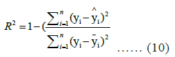
where ȳ is the mean of actual values yi. An R² value close to 1 indicates a strong model fit, while a value near 0 suggests a poor fit [33, 34].
Linear Regression, Random Forest Regressor, and Gradient Boosting Regressor were developed to predict TBM performance outcomes. The model that consistently achieved the lowest MAE, MSE, and RMSE values and the highest R² was deemed the most effective in predicting TBM performance. This model’s ability to capture non-linear relationships reinforced its suitability for complex datasets, enhancing its potential to improve predictive accuracy in TBM and geotechnical applications.
Clustering and dimensionality reduction
K-Means clustering was applied to classify different operational states, with the optimal number of clusters determined through the Elbow Method [35]. Principal Component Analysis (PCA) was subsequently used to reduce data dimensionality, allowing for clear visualization of these clusters and revealing distinct operating conditions in TBM performance [36]. Clustering facilitated the identification of operational patterns, aiding in the categorization of TBM performance under diverse geotechnical conditions [37].
K-means clustering: K-Means clustering partitions data points into k clusters by minimizing the sum of squared distances between each data point and its assigned cluster centroid. Mathematically, the objective function is:

- k is the number of clusters,
- Ci represents the i-th cluster,
- x is a data point in cluster Ci,
- μi is the centroid of cluster Ci,
- ∥x − μi∥² denotes the Euclidean distance between x and μi.
Elbow method: The elbow method was employed to determine the optimal number of clusters, k, by evaluating the Within-Cluster Sum of Squares (WCSS) for different values of k. The WCSS is computed as:
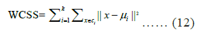
The value of k at the “elbow” point, where the decrease in WCSS becomes marginal, is selected as the optimal number of clusters.
Principal Component Analysis (PCA): Principal Component Analysis was used to reduce the dimensionality of the data, facilitating visualization of the clusters in two or three dimensions. PCA achieves dimensionality reduction by transforming the data into a set of linearly uncorrelated components, which explain the variance in the data. For each component j, the principal component score is calculated as:

Where:
- p is the original number of features,
- xi is the i-th feature,
- wij is the weight (loading) assigned to the i-th feature in component j.
The clustering analysis with the optimal k enabled clear categorization of TBM operational states [38, 39]. Visualizing clusters through PCA facilitated the understanding of different TBM performance patterns under varying geotechnical conditions. This approach provided a structured method to classify and analyze TBM operating conditions, supporting data-driven insights into TBM efficiency and operational categorization.
Results and Discussion
Mutual Information (MI) measures the dependency between two variables, capturing nonlinear relationships. Higher MI scores indicate stronger relationships, regardless of whether they’re linear or nonlinear.
Table 1 shows the Mutual Information (MI) values between several features in the dataset. Mutual Information measures the extent to which two variables share information, which may include both linear and non-linear relationships. The higher the MI value, the stronger the relationship between the feature and the target variable or between features themselves. According to the table, tensile strength has the highest MI value, 0.575929, indicating a relatively strong relationship with the target variable or other features. It is followed by uniaxial strength, with an MI value of 0.548200, which also indicates significant dependence. Spacing (0.449164) still shows a fairly strong dependence, although not as strong as tensile strength and uniaxial strength.
| No | Fitur | Mutual Information (MI) |
|---|---|---|
| 0 | Cutter Diameter | 0.356691 |
| 1 | Tip Width | 0.324788 |
| 2 | Spacing | 0.449164 |
| 3 | Penetration | 0.309554 |
| 4 | Normal Force | 0.147374 |
| 5 | Rolling Force | 0.112586 |
| 6 | Uniaxial Strength | 0.5482 |
| 7 | Tensile Strength | 0.575929 |
Table 1: Mutual information score.
Features such as cutter diameter (0.356691) and tip width (0.324788) have lower MI values, indicating a weaker relationship with the target variable or between features compared to those with higher MI values. Penetration (0.309554) also shows a lower MI value, signaling weaker dependence. Meanwhile, normal force (0.147374) and rolling force (0.112586) have the lowest MI values, meaning they share very little information with the target variable or among features.
Overall, features with higher MI values, such as tensile strength and uniaxial strength, are more relevant and can be considered more important when building models or performing further analysis. In contrast, features with low MI values, such as normal force and rolling force, show weaker relationships and may be considered for removal or further analysis to better understand their role in the dataset.
Partial Dependence Plots (PDP)
PDP show how the target variable changes with a specific feature, holding other features constant. PDPs are especially useful for interpreting complex models like random forests or gradient boosting.
Figure 4 presents a Partial Dependence Plot (PDP) illustrating the influence of three variables: Uniaxial strength, spacing, and penetration on the model’s predictions. In the first plot, an increase in uniaxial strength results in a higher predicted value, as indicated by the upward trend in partial dependence. This suggests that greater uniaxial strength has a positive impact on the model’s prediction. In the second plot, a negative relationship between spacing (distance) and the predicted value is shown. As the value of spacing increases, the predicted value tends to decrease, indicating that larger spacing may reduce the model’s output. Meanwhile, in the third plot, the penetration variable shows a sharp initial decline in partial dependence, after which changes in penetration have minimal effect on the prediction. This suggests that lower penetration values strongly influence the model’s output, but the impact diminishes as penetration increases. Small vertical lines at the bottom of each plot indicate the original data distribution for each variable, providing an overview of the data spread along the x-axis.

Figure 4: Partial dependence plots showing feature effects on model predictions.
Heatmap correlation matrix
Figure 2 is a correlation matrix heatmap, displaying the correlation coefficients between various variables related to cutter and rock properties in drilling. Each cell in the heatmap represents the correlation coefficient between two variables, with values ranging from -1 to 1. The color intensity and hue indicate the strength and direction of the correlation: Positive correlations are shown in shades of red, while negative correlations are displayed in shades of blue. Stronger correlations, whether positive or negative, are represented by darker shades, while weaker correlations appear lighter.
Key observations include:
- Cutter diameter shows a strong positive correlation with tip width (0.78) and normal force (0.75).
- Tip width is positively correlated with normal force (0.82) and rolling force (0.63), indicating that as tip width increases, both
forces also tend to increase. - Spacing has a moderate negative correlation with specific energy (-0.54), suggesting that closer spacing is associated with higher
energy efficiency. - Uniaxial strength and tensile strength exhibit a moderate positive correlation (0.66) which is expected as both are measures of
rock strength. - Penetration is negatively correlated with specific energy (-0.40) implying that increased penetration may lead to lower specific
energy requirements.
The heatmap is useful for identifying relationships between variables in drilling operations, assisting in optimization and understanding of how different parameters interact (Figure 5).

Figure 5: Heatmap correlation matrix.
Analysis of Variance (ANOVA)
The ANOVA tables for Specific energy based on parameters are as follows (Table 2):
| Source | Sum of squares | Df | F | p-value |
|---|---|---|---|---|
| Cutter diameter | 3441,47 | 7 | 10,8 | 3,20 × 10⁻12 |
| Residual cutter diameter | 14979,81 | 328 | ||
| Tip width | 2691,98 | 13 | 4,24 | 0,000002 |
| Residual tip width | 15729,3 | 322 | ||
| Spacing | 8.641,8 | 14 | 20,26 | 2,18 × 10⁻36 |
| Residual spacing | 9.779,5 | 321 | ||
| Penetration | 7.749,09 | 24 | 9,41 | 5,38 × 10⁻25 |
| Residual penetration | 10.672,19 | 311 | ||
| Normal force | 1,84 × 10⁴ | 330 | 8,01 × 1026 | 1,65 × 10⁻67 |
| Residual normal force | 3,48 × 10⁻25 | 5 | ||
| Rolling force | 1,84 × 10⁴ | 330 | 7,70 × 1026 | 1,83 × 10⁻67 |
| Residual rolling force | 3,63 × 10⁻25 | 5 | ||
| Uniaxial strength | 1,11 × 10⁴ | 40 | 11,30 | 1,11 × 10⁻39 |
| Residual uniaxial strength | 7,28 × 10³ | 295 | ||
| Tensile strength | 1,22 × 10⁴ | 49 | 11,39 | 9,38 × 10⁻44 |
| Residual tensile strength | 6,24 × 10⁻25 | 286 |
Table 2: ANOVA table for specific energy.
The ANOVA table provides an analysis of variance for multiple factors affecting various mechanical properties, including Cutter diameter, Tip Width, Spacing, Penetration, normal force, rolling force, uniaxial strength, and tensile strength. Here is an interpretation of the results:
Cutter diameter: The F-value of 10.8 and a very low p-value (3.20 × 10⁻¹²) indicate a statistically significant effect of cutter diameter on the measured outcome. This suggests that cutter diameter has a notable influence, as the probability of these results occurring by chance is exceedingly low.
Tip width: With an F-value of 4.24 and a p-value of 0.000002, Tip Width also shows a statistically significant impact on the outcome. The low p-value implies that the differences in outcomes based on Tip Width are unlikely due to random variation.
Spacing: An F-value of 20.26 and an extremely low p-value (2.18 × 10⁻³⁶) suggest a highly significant effect of spacing on the observed variable. This very low probability supports the conclusion that spacing is an important factor influencing the measured results.
Penetration: The F-value of 9.41 with a p-value of 5.38 × 10⁻²⁵ implies a significant impact of Penetration. This further demonstrates that variations in Penetration levels lead to statistically significant changes in the outcome.
Normal force: The exceptionally high F-value (8.01 × 10²⁶) and extremely low p-value (1.65 × 10⁻⁶⁷) indicate a good significant effect of normal force. This large F-value suggests a very strong relationship between normal force and the observed variable.
Rolling force: Similar to normal force, rolling force also has a very high F-value (7.70 × 10²⁶) and a p-value close to zero (1.83 × 10⁻⁶⁷), signifying a highly significant effect. This result supports the importance of rolling force in determining the outcome.
Uniaxial strength: The F-value of 11.30 and a p-value of 1.11 × 10⁻³⁹ point to a significant influence of uniaxial strength. the very low p-value indicates that variations in uniaxial strength are associated with notable changes in the measured property.
Tensile strength: With an F-value of 11.39 and a p-value of 9.38 × 10⁻⁴⁴, tensile strength exhibits a significant effect on the outcome. The probability of this result occurring by chance is extraordinarily low, confirming that tensile strength is a significant factor.
Each factor tested in the ANOVA table, as indicated by the low p-values, significantly influences the specific outcomes measured. High F-values and correspondingly low p-values across factors suggest that each has a substantial effect, with statistical significance suggesting these are not results of random variation. These findings provide strong evidence that cutter diameter, tip width, spacing, penetration, normal force, rolling force, uniaxial strength tensile strength all play significant roles in determining the observed mechanical properties in this analysis.
Performance comparison of regression models The scatter plot in Figure 6 provides a comparison of the performance metrics for three regression models: Linear Regression, Random Forest Regressor Gradient Boosting Regressor. The metrics displayed include:

Figure 6: Comparison of regression model performance metrics.
- MAE (Mean Absolute Error) in blue, representing the average absolute error in predictions.
- MSE (Mean Squared Error) in orange, which emphasizes larger errors.
- RMSE (Root Mean Squared Error) in green, showing the average magnitude of prediction errors.
- R-squared (R²) in red, indicating the proportion of variance explained by the model.
From the plot, it can be observed that the gradient boosting regressor generally performs the best across these metrics, followed by the random forest regressor, with linear regression having the highest error values and the lowest R-squared value.
The comparison performance model regression are as follows (Table 3).
| Model | Mean Absolute Error (MAE) | Mean Squared Error (MSE) | Root Mean Squared Error (RMSE) | R-squared (R²) |
|---|---|---|---|---|
| Linear Regression | 3.08 | 0,815278 | 4.35 | 0,04167 |
| Random Forest Regressor | 1.43 | 0,252778 | 2.38 | 0,06111 |
| Gradient Boosting Regressor | 1.23 | 0,214583 | 2.16 | 0,0625 |
Table 3: Comparison performance model regression.
The data in Table 3 Comparison of Regression Model Performance presents a comparison of the performance of three regression models - Linear Regression, Random Forest Regressor Gradient Boosting Regressor - based on four evaluation metrics: Mean Absolute Error (MAE), Mean Squared Error (MSE), Root Mean Squared Error (RMSE) R-squared (R²). The Gradient Boosting Regressor was found to demonstrate the strongest performance among the three models, achieving the lowest Mean Absolute Error (MAE) of 1.23, Mean Squared Error (MSE) of 0.2146 Root Mean Squared Error (RMSE) of 2.16, indicating smaller prediction errors compared to the other models. Additionally, its R2 value of 0.0625 suggests that approximately 90% of the variance in the target variable, “Specific energy hp hr/yd3,” is explained. This high performance reflects the model’s capacity to capture complex relationships in the data and generalize effectively, largely due to its sequential optimization of multiple weak learners (decision trees) that effectively reduce errors, especially in nonlinear scenarios.
The Random Forest Regressor also performed well, with an MAE of 1.43, MSE of 0.2528 RMSE of 2.38, though these values are slightly higher than those of Gradient Boosting, indicating slightly larger errors. Its R² value of 0.0611 suggests that around 89% of the variance is explained, which is good but slightly lower than that of Gradient Boosting. Random Forests are noted for minimizing overfitting by averaging multiple decision trees and perform well with nonlinear relationships; however, Gradient Boosting’s sequential approach yields greater accuracy for this dataset.
In contrast, Linear Regression served as a baseline model and produced significantly larger errors, with an MAE of 3.08, MSE of 0.8153 RMSE of 4.35. Its R² value of 0.0417 is low, indicating that only around 4.2% of the variance in “Specific energy hp_hr/yd³” is explained. The limited complexity of Linear Regression makes it less suitable for capturing nonlinear patterns in the data, resulting in lower predictive performance compared to the ensemble models.
The Gradient Boosting Regressor is recommended for this dataset due to its superior accuracy across all evaluation metrics, achieving the lowest MAE, MSE RMSE values, along with the highest R². This model effectively captures complex, nonlinear relationships, making it highly suitable for predicting “Specific energy hp_hr/yd³”.
The Random Forest Regressor also demonstrated strong performance and may serve as a good alternative if computational resources are limited, as Random Forests generally train faster than Gradient Boosting. However, in this case, Gradient Boosting provides the optimal balance between accuracy and complexity. The Linear Regression model can be used as a baseline but lacks the predictive power needed for accurate outcomes on this dataset. Its inability to capture the nonlinear patterns in the data results in higher prediction errors and a low R² value. The Gradient Boosting Regressor offers the most accurate and reliable predictions for “Specific energy hp_hr/ yd³” in this dataset, making it the most suitable model.
Optimizing clusters with the elbow method: K-means clustering, PCA visualization and cluster summary
Below are the results of applying the Elbow Method to determine the optimal value of K in the K-Means algorithm. First, the Elbow Method is used to plot a graph that helps determine the correct number of clusters by identifying the elbow point, which indicates a slower decrease in variance.
After finding the optimal number of clusters, the K-Means algorithm is used to group the data into the appropriate clusters. Next, to simplify visualization the PCA (Principal Component Analysis) method is applied to reduce the data dimensions to 2D, allowing for a clearer graphical representation of the cluster distribution. Finally, the cluster summary provides further insights into the average values for each feature within each cluster, which helps in understanding the characteristics of each group (Figure 7).

Figure 7: Elbow method for optimal K.
The Elbow Method plot is utilized to determine the optimal number of clusters (K) in a dataset for clustering algorithms such as K-means. Inertia, which represents the sum of squared distances between each data point and the centroid of its assigned cluster, is shown in the plot. Lower inertia values suggest that data points are closer to their cluster centers, indicating better-defined clusters. As the number of clusters (K) increases, inertia decreases because each cluster becomes smaller and more specific to a group of points. A significant drop in inertia is observed as K increases from 1 to 4, after which the rate of decrease in inertia slows considerably. The ‘elbow’ is typically identified at the point where this transition occurs, where adding more clusters beyond that point yields diminishing returns in reducing inertia. This point is often considered the optimal number of clusters, as it balances compactness and simplicity. In this plot, the elbow appears around K=3 or K=4, suggesting that these values could represent the optimal number of clusters for the dataset. Using more clusters may overfit the data or add unnecessary complexity without providing significant benefits. Therefore, K=3 or K=4 would provide well-defined clusters without excessive complexity. The choice between 3 and 4 may depend on specific clustering goals or further evaluation of interpretability and practicality in the application context. In summary, the Elbow Method suggests that 3 or 4 clusters would be optimal, as adding more clusters beyond this point does not significantly reduce inertia.
Clustering can be performed based on several key parameters, as outlined below. Cutter diameter, for example, can be used to group the data into categories such as small diameter (<15 mm), medium diameter (15 mm-20 mm) large diameter (>20 mm). Tip width is another parameter for clustering, with classifications like small tip width (<0.5 mm), medium tip width (0.5-0.75 mm) large tip width (>0.75 mm). Spacing between cutters can also be used for grouping, such as small spacing (<2 mm), medium spacing (2-4 mm) large spacing (>4 mm). Penetration depth is considered, with categories like shallow penetration (<0.25 mm), medium penetration (0.25-0.5 mm) deep penetration (>0.5 mm). Normal force and rolling force can be grouped based on the magnitude of the forces, with low forces (<5000 N), medium forces (5000-10000 N) high forces (>10000 N). Material strength, such as uniaxial strength and tensile strength, is another parameter for clustering, with low strength (<15000 MPa), medium strength (15000-25000 MPa) high strength (>25000 MPa). Finally, specific energy can be used to group the data into low energy (<5 MJ/m³), medium energy (5–10 MJ/m³) high energy (>10 MJ/m³) categories. These groupings provide a useful overview for analyzing trends in various cutting parameters, which can be applied to optimize processes based on specific conditions or materials (Table 4).
| No | Cutting condition | Specific energy | Normal force | Rolling force | Cluster |
|---|---|---|---|---|---|
| 0 | Condition1 | 4.269376 | 32163 | 2446 | 0 |
| 1 | Condition2 | 5.820501 | 41242 | 5002 | 1 |
| 2 | Condition3 | 5.807992 | 46634 | 6655 | 1 |
| 3 | Condition4 | 5.322232 | 51969 | 7623 | 1 |
| 4 | Condition5 | 12.03664 | 68521 | 6896 | 1 |
| ... | ... | ... | ... | ... | ... |
| 331 | Condition332 | 4.352258 | 3681.597 | 554.1077 | 0 |
| 332 | Condition333 | 6.609274 | 1841.327 | 378.6569 | 0 |
| 333 | Condition334 | 5.181177 | 2433.687 | 494.7312 | 0 |
| 334 | Condition335 | 4.807548 | 2760.189 | 550.8656 | 0 |
| 335 | Condition336 | 3.772692 | 4010.447 | 720.4804 | 0 |
Table 4: Cluster data..
The cluster data table 4 provides a summary of different cutting conditions organized by clusters. Each row represents a specific cutting condition, with key variables such as ‘Specific energy,’ ‘Normal force,’ and ‘Rolling Force,’ as well as the assigned cluster label. The dataset is segmented into multiple clusters, with Cluster 0 and Cluster 1 being the primary groups. Specific energy values are lower for Cluster 0, indicating that the cutting conditions in this cluster require less energy per unit volume. In contrast, Cluster 1 shows higher Specific energy values, suggesting that these conditions are more energy-intensive. Normal force, which represents the force perpendicular to the cutting surface, varies significantly across clusters. Cluster 0 generally has lower normal force values, while Cluster 1 exhibits considerably higher normal force values, implying that conditions in Cluster 1 require greater force. Rolling Force, which contributes to the rotational component of the cutting process, also varies between clusters, with Cluster 0 showing lower values compared to Cluster 1. Conditions in Cluster 0 are associated with lower Specific energy, normal force Rolling Force, indicating greater efficiency in terms of energy and force. Examples such as ‘Condition1,’ ‘Condition332,’ and ‘Condition336’ are assigned to Cluster 0, showing lower values for all three metrics. In contrast, conditions in Cluster 1 exhibit higher values for Specific energy, Normal force Rolling Force, indicating more demanding cutting conditions, possibly corresponding to tougher materials or more aggressive parameters. Examples like ‘Condition2,’ ‘Condition4,’ and ‘Condition5’ are assigned to Cluster 1, showing significantly higher values.
The clustering suggests that Cluster 0 conditions are more efficient, suitable for applications where energy savings and lower forces are desired, while Cluster 1 conditions, with their higher energy and force requirements, may be suited for heavy-duty or high-performance applications. This clustering can help in selecting appropriate cutting conditions based on specific energy or force constraints (Figure 8).

Figure 8: Cluster analysis of cutting conditions (PCA)
The Principal Component Analysis (PCA) plot provides a 2D visualization of the clusters identified in the dataset, resulting from dimensionality reduction. The x-axis represents Principal Component 1 the y-axis represents Principal Component 2. These components are linear combinations of the original variables, chosen to capture as much variance as possible in the data. By reducing the data to two principal components, the complexity is minimized, making it easier to visualize patterns and groupings within the dataset. The data points are color-coded based on the clusters they belong to, with each color corresponding to a specific cluster, as indicated by the color gradient on the right. Cluster 0 (green) is primarily located on the left side of the plot, suggesting that its data points share similarities in their principal component values that distinguish them from the other clusters. Cluster 1 (yellow) occupies a central position, indicating an intermediate set of characteristics between Cluster 0 and Cluster 2. Cluster 2 (purple) is positioned on the right side, indicating a distinct set of properties that differentiate it from the other clusters. The spread of points within each cluster reveals the variance in the dataset for each group. For example, Cluster 0 exhibits a wider spread along both principal components, indicating higher variance within that cluster compared to the others. While PCA helps visualize the clusters in two dimensions, some information from the original dataset is inevitably lost in this transformation. Thus, although the clusters are clearly separated in this plot, this 2D visualization may not fully capture all the complexities of the original multidimensional data. In summary, the PCA visualization demonstrates clear separation among the clusters, indicating that they have unique properties captured through dimensionality reduction.
The cluster summary provides perceptions into the average values for each feature within each cluster (Table 5).
| Cluster | Cutter diameter | Tip width (in) | Spacing | Penetration | Normal Force | Rolling Force | Uniaxial strength | Tensile strength | Specific energy |
|---|---|---|---|---|---|---|---|---|---|
| 0 | 9.444724 | 0.361156 | 2.72201 | 0.236558 | 13741.8376 | 1840.95302 | 14447.9309 | 1188.5628 | 7.124275 |
| 1 | 16.64368 | 0.556736 | 3.641839 | 0.526322 | 46201.0951 | 6841.1597 | 20156.4195 | 1417.9552 | 9.555326 |
| 2 | 8.22 | 0.357 | 1.3425 | 0.1188 | 15105.763 | 1784.23236 | 27441.72 | 1763.64 | 23.917993 |
Table 5: Cluster summary result.
The cluster summary compares three clusters based on specific drilling and mechanical properties, including cutter diameter, tip width, spacing, penetration, normal force, rolling force, uniaxial strength, tensile strength specific energy. Cluster 0 is characterized by moderate to low values across most properties, with a relatively small cutter diameter, shallow penetration low energy consumption, making it suitable for applications requiring less power and strength. Cluster 1, on the other hand, exhibits the highest values in almost all properties, including the largest cutter diameter, highest forces higher energy consumption, indicating that it is best suited for high-force applications where larger, stronger more force-intensive operations are needed.
Cluster 2 features a smaller cutter and spacing but higher material strength and energy consumption, suggesting that it is optimal for high-strength materials where the cutting force needs to be concentrated in a smaller area, resulting in higher energy demands. Overall, each cluster represents different configurations of drilling conditions tailored to specific application requirements, ranging from low-energy and moderate-strength conditions to high-force and high-strength scenarios. By comparing all the clusters, conclusions can be drawn regarding the optimal and non-optimal cutting conditions. The optimal cluster is identified as one with a combination of low specific energy and moderate or low cutting forces, suggesting more efficient and less energy-intensive conditions. Conversely, the non-optimal cluster is characterized by high specific energy or high cutting forces, which may indicate cutting conditions that require adjustments to improve performance. This approach aids in identifying the most efficient cutting conditions, providing a foundation for further experimentations or optimization of tool configurations and cutting parameters.
Conclusion
This study has successfully highlighted the performance capabilities of Earth Pressure Balance (EPB) Tunnel Boring Machines (TBMs) during the construction of the Jakarta MRT’s Underground Section CP106. Using comprehensive analysis methods such as Mutual Information (MI), Partial Dependence Plots (PDP) ANOVA, we identified several factors that significantly influence TBM efficiency, including Tensile Strength, uniaxial strength, Spacing, Penetration. The Gradient Boosting Regressor emerged as the most accurate predictive model for this dataset, effectively capturing the nonlinear relationships in TBM operational data. Additionally, clustering methods revealed distinct patterns in operational configurations, indicating that settings with lower Specific energy, normal force, Rolling Force tend to enhance energy efficiency and reduce force requirements, making them preferable for less energy-intensive tunneling.
Future research should focus on enhancing model validation by incorporating additional machine learning models and cross-validation techniques to confirm the robustness of the Gradient Boosting Regressor’s predictions. Moreover, the implementation of realtime monitoring and analysis could improve on-the-fly adjustments in TBM operations, optimizing both safety and performance. The clustering insights derived from this study also suggest that TBM configurations can be tailored to specific ground conditions, allowing for energy efficiency optimization and a reduction in mechanical wear. Lastly, integrating a broader range of geotechnical parameters, such as soil moisture content and temperature, into predictive models could enhance the accuracy of TBM performance predictions, adapting them effectively to various ground conditions encountered in tunneling projects.
References
- Sk A, Potnis DPS (2024) Enhancing urban tunnelling efficiency through real-time geotechnical parameter analysis, a case study at Kolkata East West metro project, KMRCL-1674. Int J Multidiscip Res 6:2.
[Crossref]
- Suryawan IW, Mulyana R, Septiariva IY, Prayogo W, Suhardono S (2024) Smart urbanism, citizen-centric approaches and integrated environmental services in transit-oriented development in Jakarta, Indonesia. Res Globalization 8:100181.
- Samadi H, Hassanpour J, Rostami J (2023) Prediction of earth pressure balance for EPB-TBM using machine learning algorithms. Int J Geo Engin 14(1):21.
- Zhai S, Song Y, Tian H (2024) Development of thrust, torque and power estimation model and prediction performance of earth pressure balance tunnel boring machine in mixed-face strata. Appl Sci14(13):5887.
- Wang J, Lin G, Tang R, Zhang Y, Yao Z (2024) A particle-scale insight into the face stability of shallow EPB shield tunnels in dry cobble-rich soil. Tunnel Undergr Space Techno 144:105516.
- Wang X, Li S, Li Z, Yuan C, Zhao S, et al (2024) Optimizing cutter wear in TBM operations through numerical analysis of enhanced rock-cutting interaction. Simul Model Prac Theor 2:102976.
- Fu X, Pan Y, Zhang L (2024) A Causal-Temporal Graphic Convolutional Network (CT-GCN) approach for TBM load prediction in tunnel excavation. Exp Sys Appl 238:121977.
- Fu X, Wu M, Tiong RL, Zhang L (2024) Data-driven joint multi-objective prediction and optimization for advanced control during tunnel construction. Exp Sys Appl 238:122118.
- Kilic K, Ikeda H, Narihiro O, Adachi T, Kawamura Y (2024) A soft ground micro TBM’s specific energy prediction using an eXplainable neural network through shapley additive explanation and Optuna. B Eng Geol Environ 83(5):175.
- Huang L, Zhou X, Shi L, Gong L (2024) Time series feature selection method based on mutual information. App Sci 14(5):1960.
- Keshtegar B, Hasanipanah M, Nguyen TT, Yagiz S, Bakhshandeh AH (2021) Potential efficacy and application of a new statistical meta based-model to predict TBM performance. Int J Min Rec Environ 35(7):471-87.
- Salimi A, Rostami J, Moormann C, Hassanpour J (2022) Introducing tree-based-regression models for prediction of hard rock TBM performance with consideration of rock type. Rock Mech Rock Eng 55(8):4869-91.
- Cai L, Guo X, Zhong W (2024) Test and measure for partial mean dependence based on machine learning methods. J Am Stat Ass1:1-32.
- Liang B, Liu H, Cressey EL, Xu C, Shi L, et al (2023) Uncertainty of partial dependence relationship between climate and vegetation growth calculated by machine learning models. Rem Sens 15(11):2920.
- Armstrong D (2023) Interactions and Non-Linearities in Regression Models.
[Crossref]
- Wang X, Yuan Y, Mu X, Sun W, Song X (2019) Sensitivity of TBM’s performance to structural, control and geological parameters under different prediction models. IEEE 7:19738-51.
- Walizada S (2021) Significance of correlation in statistics. Int J Multidis Res Grow Eval 2:6.
- Deng S, Zhang J, Huang Y, Zhong J, Yang X (2024) A revisit to Pearson correlation coefficient under multiplicative distortions. Comm Stat Simul Comput 27:1-23.
- Gaines SO (2023). Output regarding Creation of Correlation Matrix, Gaines et al. (2013, n = 172). 319-322
[Crossref]
- Kim KY, Jo SA, Ryu HH, Cho GC (2020) Prediction of TBM performance based on specific energy. Geomech Eng 22(6):489-96.
- Chu J, Lee TH, Ullah A, Xu H (2021) Exact distribution of the F-statistic under heteroskedasticity of unknown form for improved inference. J Stat Comp Simul 91(9):1782-801.
- Fingerhut A (2023) Probability, p values and statistical significance: Instructions for use by surgeons. British J Sur 110(4):399-400.
- Odek R, Opuodho G (2023) F-test and p-values: A synopsis. J Management Sci 13(2):59-61.
- Sil A, Betkerur J, Das NK (2019) p-value demystified. Indian Dermatol Online J 10(6):745-50.
- Park B, Lee C, Choi SW, Kang TH, Chang SH (2021) Discrete-element analysis of the excavation performance of an EPB shield TBM under different operating conditions. App Sci 11(11):5119.
- Pourhashemi SM, Ahangari K, Hassanpour J, Eftekhari SM (2021) Evaluating the influence of engineering geological parameters on TBM performance during grinding process in limestone strata. Bul Eng Geol Env 80:3023-40.
- Zhang H, Xia M, Huang F, Zhang Z (2024) Research on rock-breaking characteristics of cutters and matching of cutter spacing and penetration for tunnel boring machine. Buildings 14(6):1757.
- Ma T, Jin Y, Liu Z, Prasad YK (2022) Research on prediction of TBM performance of deep-buried tunnel based on machine learning. App Sci 12(13):6599.
- Müller PG, Lüdecke HJ (2024) Normalized coefficients of prediction accuracy for comparative forecast verification and modelling. Res Stat 2(1):2317172.
- Robeson SM, Willmott CJ (2023) Decomposition of the Mean Absolute Error (MAE) into systematic and unsystematic components. PloS one 18(2): e0279774.
- Zhang Y, Zhao Y, Wang G, Xue R (2021) Mean square cross error: Performance analysis and applications in non-gaussian signal processing. EURASIP J Adv Signal Proces 2021(1):24.
- Hodson TO (2022) Root Mean Square Error (RMSE) or Mean Absolute Error (MAE): When to use them or not. Geosci Model Develop Dis 2022:1-0.
- Ozili PK (2023) The Acceptable R-Square In Empirical Modelling For Social Science Research. Insocial Research Methodology And Publishing Results: A Guide To Non-Native English Speakers. IGI global.
- Rights JD, Sterba SK (2020) New recommendations on the use of R-squared differences in multilevel model comparisons. Multiv Behav Res55(4):568-99.
- Onumanyi AJ, Molokomme DN, Isaac SJ, Abu MAM (2022) AutoElbow: An automatic elbow detection method for estimating the number of clusters in a dataset. App Sci 12(15):7515.
- Chaouk H, Obeid E, Halwani J, Arayro J, Mezher R, et al (2024) Application of principal component analysis for the elucidation of operational features for pervaporation desalination performance of PVA-based TFC membrane. Processes. 12(7):1502.
- Wang H, Wang J, Zhao Y, Xu H (2021) Tunneling parameters optimization based on multi-objective differential evolution algorithm. Soft Computing 25:3637-56.
- Wang W, Yan C, Guo J, Zhao H, Li G, et al (2024) Improving tunnel boring machine tunnelling performance by investigating the particle size distribution of rock chips and cutter consumption. Buildings 14(4):1124.
- Zhang J, Chen M, Hong X (2021) Nonlinear process monitoring using a mixture of probabilistic PCA with clusterings. Neurocomputing 458:319-26.