Spanish
  Chinese
  Russian
  German
  French
  Japanese
  Portuguese
  Hindi
Hindi Research Article, Geoinfor Geostat An Overview Vol: 7 Issue: 1
Spatio-temporal Kriging to Predict Water Table Depths from Monitoring Data in a Conservation Area at São Paulo State, Brazil
Manzione RL1*, Takafuji EHDM2, De Iaco S3, Cappello C3 and Da Rocha MM2
1School of Sciences and Engineering, São Paulo State University (FCE/UNESP), Tupã, Brazil
2Institute of Geosciences, University of São Paulo (IGc/USP), São Paulo, Brazil
3Dipartimento di Scenze dell’Economia, University of Salento, Italy
*Corresponding Author: Manzione RL
School of Sciences and Engineering, São Paulo State University (FCE/UNESP), Tupã, Brazil
Tel: +55 14 3404-4200
E-mail: rlmanzione@gmail.com
Received: April 04, 2019 Accepted: May 27, 2019 Published: June 04, 2019
Citation: Manzione RL, Takafuji EHDM, De Iaco S, Cappello C, Da Rocha MM (2019) Spatio-temporal Kriging to Predict Water Table Depths from Monitoring Data in a Conservation Area at São Paulo State, Brazil. Geoinfor Geostat: An Overview 7:1. doi: 10.4172/2327-4581.1000205
Abstract
Abstract
The objective of this study is to explore the spatio-temporal nature of groundwater monitoring data using space-time (ST) geostatistics in order to predict water table depths at Bauru Aquifer System (BAS) in a conservation area at São Paulo State, Brazil. The information about the groundwater oscillation process in space and time can be measured in terms of spatial and temporal correlation through the ST variogram. The targets was predict water table depths in a missing date inside the monitoring period and propose a validation of these predictions based on predicted and observed values distribution curves for that specific date. Before modelling the ST empirical variogram, separability between space and time structures was checked. Then, the ST kriging predictions for March 31, 2016 were compared with independent observed dataset. ST kriging was a robust interpolator, turning possible a reasonable reconstructions of a hypothetical missing scenario inside the monitoring period in the BAS study area. The results showed a strong dependence of the temporal mean in the predictions.
Keywords: Space-time variability, Space-time interpolation
Introduction
One of the main interesting features of a geospatial network collecting water table depths monitoring data is its capacity to investigate not only the spatial distribution of the aquifer characteristics but also the temporal dynamics and variations. But modelling the spatio-temporal variability is tricky first of all because distances in space and time are not comparable. The obvious link between space and time is many times ignored by researchers due to its difficulty to join variabilities that happen in different dimensions in one single model. For Gneiting and Guttorp [1], time is intrinsically distinct from space, while time moves in only direction (forward), space do not present a preferred direction. Moreover, it is difficult (if not impossible) to compare the spatial and temporal intervals, which happen in unconnected units. In general, monitoring data have both indexations with space varying in meters, kilometres (a measure of distance) and time varying in days, months, years, centuries (a measure of existence). Furthermore Cressie and Wikle [2], explain that the modelling of space–time (ST) distributions, which come from the progress of dynamic mechanisms in space and time, is critical in many scientific and engineering fields.
Like Kyriakidis and Journel [3] comment, ST data were first analysed through models that were developed originally for temporal or spatial distributions. The joint space–time correlation is nowadays fully modelled for prediction/forecasting purposes through the use of various ST variogram models available in the literature [4-9]. Although the selection of an appropriate class of models could be based on its geometric features and theoretical properties [9,10], in practice, the generalized product–sum model by De Iaco et al. [11] is largely used in different areas, ranging from environmental sciences to medicine and from ecology to hydrology [12-17].
As an extension of traditional geostatistics, ST geostatistics has all its the advantages of making optimal estimations with the available dataset, computing the accuracy of the estimations/predictions, considering the covariate information and offering adaptability in modelling [18]. The computation is similar, however calculation can take longer due to the usually large conditioning datasets, making estimation grid also large, especially, with the addition of an extra dimension. Moreover, Gräler et al. [19] discuss that it is possible to estimate values pondering the spatial and temporal neighbouring observations from spatial and temporal correlations. ST interpolation can potentially compute more accurate estimations/predictions than purely spatial interpolation due to the consideration of the observations taken at other times.
As Heuvelink et al. [20] stated, the widespread collection of valid space-time covariance functions structures developed in the last decades followed by practical side publications and more userfriendly software solutions increased the use of ST geostatistics. Many applications of ST geostatistics are mentioned in the literature, varying from field like agriculture [21], air quality [22,23], climatology [24,25], soil science [26,27], health [28], ecology [29], among others. Especially on hydrogeology, it is worth recalling early works like Rouhani and Hall [30] which describe the application of space-time kriging of groundwater data and Rouhani and Myers [31] which state some problems when using ST kriging for some typical configurations of hydrological data. In recent studies, Júnez-Ferreira and Herrera [32] used ST kriging to water level estimation of the Queretaro- Obrajuelo aquifer in Mexico, while Varouchakis and Hristopulos [33] performed a comparison between spatio-temporal variogram functions on scarce information of groundwater level oscillation in the isle of Creta, Greece. As Varouchakis and Hristopulos [33] highlighted, there are some difficulties when applying these methods for groundwater datasets because hydrogeological data based on insitu metering are frequently sparse in space and dense in time, what can introduce a significantly different levels of reliability in space and time. The validation of ST kriging methods is not discussed in practical terms and there is a lack of studies comparing predictions and forecasts with future observations.
The objective of this research is to verify the applicability of ST geostatistics to predict water table depths from hydrogeological monitoring data in a conservation area in the Brazilian Cerrado. Observed levels are compared with predicted levels for a time instant inside the monitoring period in order to evaluate ST kriging performance. It is proposed a framework to analyse ST kriging water table depths predictions based on its distribution functions compared with observed values and on errors measurements.
Space-time Geostatistics
Two major conceptual viewpoints for modelling spatiotemporal distributions via spatial statistics tools extended to include the additional time dimension were defined by Kyriakidis and Journel [3]. Firstly, given a spatio-temporal random field  , where S is the spatial domain and T is the time interval, with finite first and second order moments, it is assumed that Z is composed by a trend component, that represent the global variability of the spatio-temporal process, and its higher frequency fluctuations as the stationary residuals:
Z(s,t) = m(s,t) + ε(s,t) (1)
where m(s,t) is a deterministic trend, which is assumed constant in space and time, or it is function of known explanatory variables (covariates) and ε (s,t) is a zero-mean stochastic residual.
In the case of water table depths, it may be reasonable to use porosity and the time of the year as explanatory variables, to support that groundwater has a seasonal oscillation and tends to fluctuate more or less according to water infiltration. The zero-mean stochastic residual ε is often assumed to be multivariate normally distributed; hence a covariance function C can describe it. This function computes the covariance between ε (s,t) and ε (s0,t0) for any pair of points (s,t) and (s0,t0) in the spatio-temporal domain. Assuming the second-order stationarity, the function depends entirely on the spatial separation lag (h=s-s0) and the temporal separation lag (u=t-t0) between the points:
 (2)
(2)
The ST trend function m(s,t) can be straightforwardly decomposed as the sum of its components (purely spatial and purely temporal) trends [1]. When h represents the Euclidean distance  the spatial isotropy assumption is considered [18].
Spatio-temporal Covariance Models
The reliability of geostatistical estimation and/or simulation results depends on the adequacy of the selected ST correlation model for the variable under study [10]. In practice, it is usual to choose a correlation model from a collection of valid known models and verify whether it fits.
In the literature there are various spatio-temporal covariance models, such as the separable/linear model [30,34,35], the product model [36], the product-sum model [37], the metric model [38,39], the Cressie-Huang model [4], the Gneiting models [6], the integrated product-sum model [5,12], and others non-separable spatio-temporal covariance models [8,40-43]. For further information about spatiotemporal geostatistics models we recommend [1,2,9,24,44,45].
When selecting an appropriated model it is important to have in mind the main features of a covariance function/variogram; among these characteristics, it is worth mentioning the separability/nonseparability between space and time.
According to the definition in De Iaco et al. [45] a second order stationary spatio-temporal random field Z has a separable covariance if there exist purely spatial Cs(h) and purely temporal CT(u) covariance functions, such that:
C(h,u)=Cs(h)CT(u) (3)
Otherwise, the ST covariance function is non-separable. Note that the separability condition can be written equivalently as
Hence, when the equality in (3) is true, one can see that the space-time covariance function can be detached into the product of a purely spatial covariance and a purely temporal covariance. Another characteristic of spatio-temporal covariance function is full symmetry:
C(h,u) = C(-h,u) = C(h,-u) = C(-h,-u) (4)
Note that a separable covariance must be fully symmetric, but full symmetry does not imply separability [46-48].
Study Area and Dataset
Santa barbara ecological station
This paper presents a spatio-temporal geostatistical analysis of data collected from Santa Barbara Ecological Station (EEcSB), a “strict nature reserves” area, or category 1a under the International Union for the Conservation of Nature and Natural Resources (IUCN). This entails severely restricted the human use and visitation of the area in order to protect the biodiversity and conservations values of the area [49]. The EEcSB was established in 1984 and is located in the municipality of Águas de Santa Bárbara, coordinates 22°48’59” S and 49°14’12” W (Figure 1).

Figure 1: Bauru Aquifer System (BAS) domain at São Paulo State, Brazil, and localization of the study area.
This reserve borders the city of Águas de Santa Bárbara to the north and covers 2,715 ha of ecologically important land [50]. It is located in the Médio Paranapanema hydrographic region, in the Paranapanema watershed. The local relief is composed primarily of wide and short hills, with altimetry around 600 and 680 m. The main soil types present in the EEcSB are Red Latosols (LV56) and eutrophic and dystrophic Red-Yellow and Red Argisols (PVA10) with sandy/ medium texture and eutrophieric Nitosols (NV1) with clay texture [51].
According to Köeppen classification, the characteristic climate of the region is tropical subhumid (Cwa-warm climate with dry winter). The average temperature is around 18°C and ranging from 16°C to 23°C in the monthly mean [52]. The annual precipitations are around 1,000 and 2,086 mm and can reach 30 mm monthly in winter [53].
Local hydrogeology and monitoring water table depths network
EEcSB is situated on the Paraná Basin, an intracratonic sedimentary basin that evolved on the South American Platform, composed of sedimentary, volcanic and basaltic rocks and drained by the Parana River, its major river. The top layer is composed by Cretaceous sandstones known as the Bauru group [54] with an average thickness of 100 m.
The Bauru Aquifer System (BAS) overlays the Serra Geral Formation, which consists of the impermeable substrate formed overtop of the Guarani Aquifer System (GAS). Groundwater recharge in this area occurs by direct infiltration as a result of precipitation in the horizontal extension of the aquifer. In some locations fractures in the Serra Geral Formation can cause leakage from BAS into the GAS [55]. At EEcSB, the geology is composed, basically, by sandstones of Bauru Group (Adamantina and Marilia Formations) and basalts (extrusive igneous rocks) from Serra Geral Formation of São Bento Group. BAS is a free aquifer, denoted as high risk to contamination due to land use and soil management, and is extensively utilized in public drinking water distribution systems [55]. Uncontrolled use of this reservoir, without rules or regulation, could change the status of the BAS from strategic drinking water reserve to a depleted water body, which could become a source of conflict in the future.
Water table depths were observed in the EEcSB at 55 monitored wells from September 5, 2014, until December 13, 2017. The wells have depth, ranging from 2.94 to 7.68 m. Figure 2 shows the layout of the wells in the study area.

Figure 2: Water table monitoring network installed at the main watersheds of Santa Barbara ecological station and state forrest.
Water Table Depths ST Modelling
ST variogram estimation and separability checking
In order to estimate the spatio-temporal variability of water table depths in the EEcSB, we selected a period covering three hydrological years (from September 05 2014 to September 04 2017) of monitoring series at 55 wells. The observed values were modelled and resampled for a semi-monthly frequency using a time series model implemented in the Menyanthes software [56].
First, the time series collected in the geospatial monitoring network were transformed into a spatio-temporal full dataframe (STFDF). Then, a ST variogram is estimated. The criteria for experimental variogram construction for both space and time dimensions follow the proposition of Journel and Huijbregts [57] that recommend using one half of the sample field (L=5,000 m) length as a limit of reliability for the estimator (cutoff |h| <L/2).
Second, we check for separability between space and time for a proper model selection. Variogram properties testing like symmetry and separability is describeb at Li et al. [46] and Cappello et al. [48]. Considering the observation taken at the same spatial points over a period of time, the null hypotheses of full symmetry and separability of a space-time, given in terms of covariance function, are presented as:
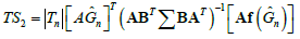
H0:AF(G)=0 (5)
where A is a contrast matrix of row rank q and f=(f1,…..fr)T are realvalued functions that are differentiable at  the vector of covariances at the specified lags in Λ. If
  with
with , denote the covariance estimators based on random variables in the sequence of the index sets,
  with a fixed space
  and regularly spaced times Tn={1,…..,n}, and let
  is the estimator G computed over Dn. In case of symmetry (f(G)=G), the null hypothesis is frequently written as. H0:AG=0As a consequence, the suggested statistical analysis for verifying symmetry and separability are respectively:
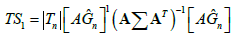 (6)
(6)
 (7)
(7)
and, under, H0 they converge in distribution to a chi-square with q degrees of freedom. The generic element of the matrix B is, 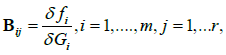 with fj and Gi the j-th component of f and the i-th component of G, respectively. By simplicity, it is assumed that the expectation of Z is known and equal to zero. Nevertheless, if this assumption is disregarded, it is enough to denote with with
 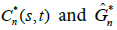 the mean-corrected estimators of C(s,t) and G, since
 have the same asymptotic properties. More details can be found in Li et al. [46] and Cappello et al. [48].
Third, ST variability is modelled using a model that suits to the tested hypothesis of separability. Note that separability test can be performed using the package covatest [58] and ST variogram calculations can be performed using the packages gstat [59] and spacetime [60], all from R software [61].
Water Table Depths ST Prediction
ST kriging
Usually, before performing the ST kriging, the global trend should be modelled, and the stochastic residual covariance function should be computed. Then, the spatio-temporal kriging can be calculated as traditional ordinary kriging functions. If the trend is a linear function of covariates, then Kriging with External Drift (KED) is the most appropriate approach [62].
In the following the ordinary kriging algorithm (constant and unknown deterministic component) was used to interpolate an instant within the time series whose observations were not used to construct the variogram. The date of March 31, 2016 was selected as the target and later field observations of that date were used to validate the generated map. ST kriging was also performed using the R packages gstat and spacetime.
ST model validation
To evaluate the ST kriging performance on predict water table depths, after variogram modelling and ST interpolation we estimated distribution functions and cumulative distribution functions for observed and predicted water table depths at March 31, 2016. The distribution functions were estimated using the values observed in the monitoring wells specifically in this date and, for the same locations, the values estimated using ST kriging. The Kolmogorov– Smirnov test (KS test) was used for comparing two-by-two samples, with the null hypothesis that the samples are drawn from the same distribution, independently of the interpolation method [63,64].
Results and Discussion
Separability test and ST variogram modelling
The ST variogram from September 05, 2014 to September 04, 2017 was calculated using 38 time steps (18 months) once it was considered half of the temporal field. The parameters of the ST variogram are presented in Table 1 and the resulting experimental ST variogram presented in Figure 3.
| ST variogram | Cutoff | Width |
|---|---|---|
| Space (meters) | 2,400.00 | 230.00 |
| Time (days) | 38.00 | 15.00 |
Table 1: Parameters of the experimental ST variogram for water table depths calculated for the period from September 05, 2014 to September 04, 2017 at EEcSB.

Figure 3: Experimental ST variogram for water table depths monitored from September 05, 2014 to September 04, 2017 at EEcSB.
Then, the separability assumption was verified by choosing couples of spatial points at the shortest distance ||h|| and fixing the first temporal lag, where the correlation is strong. The null hypothesis of separability is not rejected (TS=6.37 and p-value=0.496), consequently, it is reasonable to fit a separable model to the empirical variogram surface and then use this model to perform ST modelling and estimation.
Note that the separable model in terms of variogram can be written as:
 (8)
(8)
where  and
and are standardised spatial and temporal variograms with separate nugget effects and (joint) sill of 1 and k=min(sills,sillt). This function is also fully symmetric as explained by Gneiting [6], Stein [42] and De Iaco et al. [45].
The fitted separable product model is such that the spherical model (with range equal to 1,500 meters and sill 0.75) is used for the spatial component and the exponential model (with range equal to 30 days and sill 1.55) is applied for the temporal one. The results of the ST variogram adjustment are illustrated in Figure 4.

Figure 4: ST plot (left) and adjusted product model (right) for water table depths monitored from September 05, 2014 to September 04, 2017 at EEcSB.
As shown in Figures 3 and 4, in the temporal dimension the variance increases abruptly after a few moments while in the spatial dimension the variation is smoother. In the temporal dimension, the variance is greater than in the spatial dimension, with modelled sill values of 1.55 and 0.75, respectively. However, the spatial range is greater than the temporal range, showing a greater continuity of the water table oscillation process in the space from the data variation whose variance increases gradually to approximately 1,500 m and stabilizing from this distance. Whereas the variance in the time rises abruptly already in the initial times of the process and stabilizes already starting from 30 days. These values denote a water table oscillation process gradual and continuous in space and highly variable in time due to its seasonality and the monitoring network of shallow water table levels. Besides that, the spatial and temporal ranges cannot be compared numerically by different dimensions and units (space in meters and time in days). As can be seen in the ST plot, after around 150 days and 1,000 m the variation is completely random.
In general, the EEcSB groundwater system has a short memory and rapid response. In other words, it is influenced by nearby time instants whose influence tends to be lost quickly. Noticeable fluctuations in the groundwater level can be observed in the riparian zone, in space and time, evidencing a clear river influence [64]. A precipitation event, for example, would exert a rapid and strong reaction in the water table, but would not be sustained for long, due to local drainage and runoff conditions or even the incidence of new precipitation events that would exert a new and maybe even stronger influence in the levels than the previous event. In regions with widespread shallow water tables, the need to understand the drivers of its fluctuating levels becomes critical for agricultural planning and hydrological management [65].
Water table depths prediction
Thus, once determined water table depths response characteristics in space and time, the product model fitted to the data was used to predict water table depth at March 31, 2016, resulting in the map showed in Figure 5. The interpolated values presented a smooth and gradual variation in the study area, representing the same variations observed in the field with values denoting more superficial levels in the head of the Bugre, Guarantã and Passarinho watersheds. Next to the water dividers the values found were deeper, but still considered superficial (> -2.0 m).

Figure 5: Water table depths predicted for March 31, 2016 at EEcSB using ST kriging interpolation.
For Appels et al. [66], groundwater dynamics can be related with microtopographical and mesotopographical features, those that can be characterized deterministically, e.g., resulting from tillage or vegetation structure, and erratic ones such as macrofauna burrows. These features can definitely influence patterns of ponding and surface runoff in areas with small topographic gradients [67]. In the plains of Argentine Pampas, Mercau et al. [65] verified that at the inter-annual scale the water table oscillation were dominated by the variability of the climate system while the farming crop had impact on the growing season and subtle influence on the year to year oscillation. These statements reinforce the need for prediction methods capable to estimate spatial variation, accounting also for temporal variations in area where seasonality is strong and evident.
In areas where no well information was available, lower values were assigned (red map areas). These values are close to the average of the set of data used for map validation, presented in Table 2. These statistics were calculated using 55 observed and interpolated values.
| Values | All data | Obs | Stk |
|---|---|---|---|
| Minimum | -6.21 | -1.95 | -1.46 |
| 1st Quantile | -1.78 | -1.32 | -1.33 |
| Median | -1.35 | -0.89 | -1.24 |
| Mean | -1.08 | -0.63 | -1.23 |
| 3rd Quantile | -0.44 | -0.45 | -1.14 |
| Maximum | 0.32 | -0.35 | -1.03 |
Table 2: Descriptive statistics of the complete dataset, observed values at March 31, 2016 and predicted water table depths using ST kriging.
The mean, median, quantiles, minimum and maximum values, standard deviation, variance, skewness and kurtosis were not similar when comparing observed values and ST kriging predictions. Figure 6 presents the density distribution functions of observed and predicted values. The interpolated values smooth the distribution, with minimum and maximum values smaller than observed values. Also, the skewness and kurtosis denote slightly differences in the distributions. ST kriging predictions followed the premises of kriging algorithm showing normal distributed values with minimum variance and honouring the mean of the population [57,62]. Since there was no spatial mean for the predicted date, the ST kriging algorithm based its estimations in the global mean of the dataset, creating a mean scenario based on all observed time steps instead of condition its predictions to previous and further moments of the predicted date March 31, 2016.

Figure 6: Density distribution functions for observed water table depths at March 31, 2016 (red) and predicted values for the same date using ST kriging (green).
When running ST kriging, even with further points in space and time when we are making a prediction of a time frame between observations, this prediction is too attached at the mean of the whole dataset, once the variations between observations can be large. In the case of the variogram showing a pure (or almost) nugget effect in time, the results of each point will tend to average the values of each time series used in the search neighbourhood. Therefore, the density function resulting from the spatio-temporal method has a confinement around the mean. This is the inverse of the problem that was presented by Rouhani and Myers [31], where the authors report the fact of a temporal sampling larger than the spatial could cause deviations in the estimates. In this case, the estimates were based largely on the temporal mean of the process, although the network of 55 water table observation wells was considered a large dataset for a small area. Figure 7 shows cumulative distribution functions (CDF) calculated for observed and predicted values. The median values (dashed vertical lines) were far from each other, and the ST kriging CDF (green line) presented much less variability than the observed water table depths CDF (red line). ST kriging CDF presents a much narrow interval and a displacement of the median to the left.

Figure 7: Cumulative distribution functions (CDF) calculated from the observed (red) and estimated (green) water table depths for March 31, 2016 and its respective medians (dashed vertical lines).
Table 3 present error measures and the result of Kolmogorov Smirnov test for both distributions. These diagnostics denote the observed and predicted water table depths at March 31, 2016 do not belong to the same distribution. For 55 values, KS test D statistics and associated p-value rejects the null hypothesis that the sample of predicted values is drawn from the reference distribution of observed water table depths. However, mean errors (ME), mean absolute errors (MAE) and root mean squared errors (RMSE) are considered small for this kind of mapping, but large if considered the amplitude of variance contained in the data. The errors are close to the standard deviation values of the observed and predicted water table depths.
| Variables | Pred-Obs |
|---|---|
| ME | -0.36 |
| MAE | 0.51 |
| RMSE | 0.57 |
| KS (D) | 0.67 |
| p-value | 3.24E-06 |
Table 3: Errors calculated from observed and predicted water table depths for March 31, 2016.
When the aim of a spatio-temporal exercise is to predict a missing frame inside a monitoring period, like in this study, it is important to have in mind the final use of the resulting map. Errors smaller than 0.6 m are manageable errors for many agricultural groundwater purposes like pumping or drainage, but critical for others like irrigation and phreatic control. Authors like Wang et al. [64] consider shallow groundwater as an important source of water, which necessitates a deeper understanding of its complex spatial and temporal dynamics driven by hydrological processes, especially in arid environments. Tillage, crop yields and water consumption at lowlands characterized by shallow ground-water levels are affected by the groundwater levels, which therefore influence the potential to use the land for agriculture [68].
When the study objective is to forecast (predict the future from the past), Heuvelin et al. [18] recommended that the model should incorporate the driving forces and it can be done with a dynamic state-space approach (i.e. Kalman filter). One should notice that kriging methods were originally created to interpolate, thus it cannot be reliable to extrapolate beyond the ST domain of the conditioning dataset. As Cressie and Huang [4] comment, the separable ST covariance is frequently assumed due to its simplicity (reduced number of parameters that need to be estimated and ease estimation) and implies that the spatial structure is the same at all time points and the temporal structure is the same at all locations. Besides that, Montero et al. [44] argue that the separable models have been the most widely used in geostatistical application, even in situations when this hypothesis was not justified by the very nature of the process under analysis due to the product of purely spatial and purely temporal covariances permits more efficient inferences in terms of computing. However, as De Iaco [10] explains, separability is restrictive and often requires unrealistic assumptions because it does not model ST interaction. ST kriging is also promising for persistent phenomena, with long memory or even directional spatial continuity, like groundwater contamination and transport as several studies published in the field of atmospheric pollution suggest [19,22-25].
Conclusion
The application of ST geostatistical methods to water table monitoring data made it possible to explore the relationships existing in space during the period studied, relating the spatial and temporal variations by means of covariance functions. From the establishment of these data based functions was verified that there is a separable spatio-temporal behaviour in water table depths oscillation processes in the Bauru Aquifer System at EEcSB. This spatio-temporal behaviour has been well captured by the product ST variogram model, denoting a groundwater system with short memory and fast response in time and continuous variation in space. Also, It has been possible to predict water table depths for a missing frame inside the monitoring period using the modelled separable product covariance function. ST kriging predictions have been too attached to the global mean of the dataset, however the estimates did not reproduce well the observed values distribution for March 31, 2016. Errors from observed and predicted water table depths have been considered small. For shallow groundwater systems with short memory, influenced by seasonality and with fast response to localized meteorological events it is important to check significance of ST kriging predictions to avoid misinterpretations and further water management complications.
Funding
This research is funded by FAPESP (São Paulo Foundation for Scientific Research-Brazil)-Grant 2016/09737-4.
References
- Gneiting T, Guttorp P (2010) Continuous parameter spatio-temporal processes. In: Gelfand AE et al. (eds) Handbook of spatial statistics. Chapman & Hall/CRC Press, Boca Raton. pp: 427-436.
- Cressie N, Wikle CK (2010) Statistics for spatio-temporal data. Wiley.
- Kyriakidis PC, Journel AG (1999) Geostatistical space-time models: A review. Math Geol 31:651-684.
- Cressie N, Huang HC (1999) Classes of nonseparable, spatio-temporal stationary covariance functions. J Am Stat Assoc 94:1330-1340.
- De Iaco S, Myers DE, Posa D (2002a) Nonseparable space-time covariance models: Some parametric families. Math Geol 34:23-42.
- Gneiting T (2002) Nonseparable, stationary covariance functions for space-time data. J Am Stat Assoc 97:590-600.
- Ma C (2003) Spatio-temporal stationary covariance models. J Multivariate Anal 86:97–107.
- Rodrigues A, Diggle PJ (2010) A class of convolution-based models for spatio-temporal processes with non-separable covariance structure. Scand J Stat 37:553-567.
- De Iaco S, Posa D, Myers DE (2013) Characteristics of some classes of space–time covariance functions. J Stat Plan Infer 143:2002–2015.
- De Iaco S (2010) Space-time correlation analysis: A comparative study. J Appl Stat 37:1027-1041.
- De Iaco S, Myers DE, Posa D (2001) Space-time analysis using a general product-sum model. Stat Probabil Lett 52: 21–28.
- De Iaco S, Myers DE, Posa D (2002b) Space-time variograms and a functional form for total air pollution measurements. Comput Stat Data An 41:311-328.
- Myers D (2002) Space–time correlation models and contaminant plumes. Environmetrics 13: 535-553.
- Fernández-Casal R, González-Manteiga W, Febrero-Bande M (2003) Flexible spatio-temporal stationary variogram models. Stat Comput 13:127-136.
- Gething PW, Atkinson PM, Noor AM, Gikandi PW, Hay SI, et al. (2007) A local space–time kriging approach applied to a national outpatient malaria data set. Comput Geosci 33:1337–1350.
- Skøien JO, G. Blöschl G (2006) Catchments as space-time filters ? a joint spatio-temporal geostatistical analysis of runoff and precipitation. Hydrol Earth Sys Sci 10:645-662.
- Spadavecchia L, Williams M (2009) Can spatio-temporal geostatistical methods improve high resolution regionalisation of meteorological variables? Agric For Meteorol 149:1105-1117.
- Heuvelink GMB, Pebesma EJ, Gräler B (2017) Space-time geostatistics. In: Shekhar S, et al. (ed) Encyclopedia of GIS, 2nd edn. Springer, Belin. pp 1919-1926.
- Gräler B, Pebesma EJ, Heuvelink GMB (2016) Spatio-Temporal Geostatistics using gstat. R J 8:204-218.
- Heuvelink GBM, Griffith DA, Hengl T, Melles SJ (2012) Sampling Design Optimization for Space-Time Kriging. In: Mateu J, Muller WG (eds) Spatio-temporal Design: Advances in Efficient Data Acquisition. Wiley, Hoboken, pp 207–230.
- Heuvelink GBM, van Egmond FM (2010) Space-time geostatistics for precision agriculture: A case study of NDVI mapping for a Dutch potato field. In: Oliver MA (ed) Geostatistical applications for precision agriculture. Springer, Berlin, pp. 117–137.
- Paci L, Gelfand AE, Holland DM (2013) Spatio-temporal modeling for real-time ozone forecasting. Spat Stat 4:79-93.
- Monteiro A, Menezes R, Silva ME (2017) Modelling spatio-temporal data with multiple seasonalities: The NO2 Portuguese case. Spat Stat 22:371-387.
- Gneiting T, Genton MG, Guttorp P (2007) Geostatistical space-time models, stationarity, separability and full symmetry. In: Finkenstaedt B, et al. (ed) Statistics of Spatio-Temporal Systems. Chapman & Hall/CRC Press, Boca Raton, pp 150-175.
- Kilibarda M, Hengl T, Heuvelink GBM, Gräler B, Pebesma EJ, et al. (2014) Spatio-temporal interpolation of daily temperatures for global land areas at 1 km resolution. Geophys Res-Atmos 119:2294–2313.
- Snepvangers JJJC, Heuvelink GMB, Huisman JA (2003) Soil water content interpolation using spatio-temporal kriging with external drift. Geoderma 112:253–271.
- Jost G, Heuvelink GBM, Papritz A (2005) Analysing the spacetime distribution of soil water storage of a forest ecosystem using spatio-temporal kriging. Geoderma 128: 258–273.
- Mugglin AS, Cressie N, Gemmell I (2002) Hierarchical statistical modelling of influenza epidemic dynamics in space and time. Stat Med 21:2703–2721.
- Denham A, Mueller U (2010) Incorporating survey data to improve space-time geostatistical analysis of king prawn catch rate. In: Atkinson PM, Lloyd CD (eds) geoENV VII – Geostatistics for Environmental Applications. Springer, Dordrecht. pp 13-27.
- Rouhani S, Hall, TJ (1989) Space-time kriging of groundwater data. Geostatistics 4: 639-650.
- Rouhani S, Myers DE (1990) Problems in space-time kriging of hydrogeological data. Math Geol 22:611-623.
- Júnez-Ferreira HE, Herrera GS (2013) A geostatistical methodology for the optimal design of space–time hydraulic head monitoring networks and its application to the Valle de Querétaro aquifer. Environ Monit Assess 185:3527–3549.
- Varouchakis EA, Hristopulos DT (2017) Comparison of spatiotemporal variogram functions based on a sparse dataset of groundwater level variations. Spat Stat: In press.
- Bogaert P (1996) Comparison of kriging techniques in a space-time context. Math Geol 28:73–86.
- Christakos G, Bogaert P (1996) Spatio-temporal analysis of spring water ion processes derived from measurements at the Dyle basin in Belgium. IEEE T Geosci Remote 34:626–642.
- De Cesare L, Myers DE, Posa D (2001) Estimating and modeling spacetime correlation structures. Stat Probabil Lett 51: 9–14.
- De Iaco S, Myers DE, Posa D (2001) Space-time analysis using a general product-sum model. Stat Probabil Lett 52: 21–28.
- Dimitrakopoulos R, Luo X (1994) Spatio-temporal modelling: covariance and ordinary kriging systems. In: Dimitrakopoulos R (ed) Geostatistics for the next century. Kluwer Academic, Dordrecht. pp 88-93.
- Soares A, Pereira MJ (2007) Space-time modelling of air quality for environmental-risk maps: A case study in South Portugal. Comput Geosci 33:1327-1336.
- Ma C (2002) Spatio-temporal covariance functions generated by mixtures. Math Geol 34:965–975.
- Kolovos A, Christakos G, Hristopulos DT, Serre ML (2004) Methods for generating non-separable spatiotemporal covariance models with potential environmental applications. Adv Water Resour 27:815-830.
- Stein ML (2005) Space-time covariance functions. J Am Stat Assoc 100:310-321.
- Porcu E, Mateu J, Saura F (2008) New classes of covariance and spectral density functions for spatio-temporal modelling. Stoch Env Res Risk A 22:65-79.
- Montero JM, Fernandez-Aviles G, Mateu J (2015) Spatial and spatio-temporal geostatistical modeling and kriging. Wiley.
- De Iaco S, Palma M, Posa D (2016) A general procedure for selecting a class of fully symmetric space-time covariance functions. Environmetrics 27:212–224.
- Li B, Genton MG, Sherman M (2007) A nonparametric assessment of properties of space-time covariance functions. J Am Stat Assoc 102:736–744.
- Sherman M (2011) Spatio statistics and spatio-temporal data: Covariance functions and directional properties. Wiley.
- Cappello C, De Iaco S, Posa D (2018) Testing the type of non-separability and some classes of space-time covariance function models. Stoch Environ Res Risk Assess 32:17–35.
- Dudley N (2008) Guidelines for applying protected area management categories. International Union for Conservation of Nature
- Meira-Neto J, Martins F, Valente G (2007) Floristic composition and biological spectra in Santa Barbara ecological station, Brazil. Revista Árvore 31:907-922.
- Oliveira JB, Camargo MN, Rossi M, Calderano Filho B (1999) Pedological map of São Paulo State 1:500,000. Instituto Agronômico de Campinas/Fundação de Auxílio à Pesquisa do Estado de São Paulo.
- Alvares CA, Stape JL, Sentelhas PC, Golçalves JLM, Gerd S (2013) Köppen's climate classification map for Brazil. Meteorol Z 22: 711–728.
- Melo ACG, Durigan G (2011) Santa Barbara ecological station management plan. Instituto Florestal do Estado de São Paulo.
- Wendland E, Rabelo J, Roehrig J (2004) Guarani aquifer system - The strategical source in South America. Technol Resour Manag Dev 3: 192–201.
- Santos T, Bonotto D (2004) 222Rn, 226Ra and hydrochemistry in the Bauru aquifer Ssystem, São José do Rio Preto (SP), Brazil. Appl Radiat Isotopes 86:109-117.
- Manzione RL (2018) Physical-based time series model applied on water table depths dynamics characteristics simulation. Brazilian Journal of Water Resources 23:1-20.
- Journel AG, Huijbregts CJ (1978) Mining geostatistics. Academic Press.
- De Iaco S, Cappello C, Posa D (2017) Covatest: Tests on properties of space-time covariance functions.
- Pebesma EJ (2004) Multivariable geostatistics in S: The gstat package. Comput Geosci, 30:683-691.
- Pebesma EJ (2012) spacetime: Spatio-temporal data in R. J Stat Softw 51:1–30.
- R Development Core Team (2017) R: A Language and Environment for Statistical Computing. R Foundation for Statistical Computing. R Development Core Team.
- Goovaerts P (1997) Geostatistics for natural resources evaluation. Oxford University Press.
- Chakravart IM, Laha RG, Roy J (1967) Handbook of methods of applied statistics. Wiley.
- Wang P, Yu J, Pozdniakov SP, Grinevsky SO, Liu C (2014) Shallow groundwater dynamics and its driving forces in extremely arid areas: A case study of the lower Heihe River in Northwestern China. Hydrol Process 28:1539-1553.
- Mercau JL, Nosetto MD, Bert F, Giménez R, Jobbágy EG (2016) Shallow groundwater dynamics in the Pampas: Climate, landscape and crop choice effects. Agr Water Manage 163:159-168.
- Appels WM, Bogaart PW, Van der Zee SEATM (2017) Feedbacks between shallow groundwater dynamics and surface topography on runoff generation in flat fields. Water Resour Res 53:10336–10353.
- Darboux F, Davy P, Gascuel-Odoux C, Huang C (2002). Evolution of soil surface roughness and flowpath connectivity in overland flow experiments. Catena 46:125-139.
- Dietrich O, Fahle M, Seyfarth M (2016) Behavior of water balance components at sites with shallow groundwater tables: Possibilities and limitations of their simulation using different ways to control weighable groundwater lysimeters. Agr Water Manage 163:75-89.