Research Article, Geoinfor Geostat An Overview Vol: 6 Issue: 3
Visualization of Landsat Image Spectral Space as a Method of Boreal Ecosystems Geomatic Modeling (on the Example of Eastern Fennoscandia)
Litinsky Peter*
Northern Water Problems Institute KarRC, Russia
*Corresponding Author : Litinsky P
Northern Water Problems Institute KarRC RAS, Petrozavodsk, Russia
Tel: +78142576381
E-mail: litinsky@sampo.ru
Received: August 17, 2018 Accepted: August 30, 2018 Published: September 07, 2018
Citation: Litinsky P (2018) Visualization of Landsat Image Spectral Space as a Method of Boreal Ecosystems Geomatic Modeling (on the Example of Eastern Fennoscandia). Geoinfor Geostat: An Overview 6:3. doi: 10.4172/2327-4581.1000183
Abstract
A new approach to information extraction from Landsat TM/ETM+ imagery is proposed. It involves transformation of image space into a visible 3D form and comparison of positions of the ecosystem signatures in this space with graphical expression of forest and mire cover typology (biogeocenotic scheme). The model is built in the LC1-LC2-MSI axes: the two first principal components of the image matrix in logarithmicm form and moisture stress index. Compared to Tasseled Cap, this transformation is more suitable for the study area. The spectral classes of mature forests line up from the ecological optimum (moraine hills) along two main environmental gradients are : i) lack of water and nutrition (fluvioglacial sandsbedrock) and ii) degree of paludification (lacustrine plains). Thus, the biogeocenotic complexes (Quaternary deposits + vegetation) are identified. The succession trajectories of forest, regeneration through spectral space are also associated with the type of Quaternary deposits. For open mires spectral classes reflect the type of water and mineral nutrition (ombrotrophic or mesotrophic) and the level of water table. The spectral model is a mathematically formalized object that describes the quantitative and qualitative characteristics of the ecosystems. Being deployed in geographical space, it turns into the optimal structural base for integrating the results of discrete field observations into a single space-time continuum. The spectral space model created using measured by the scanner physical characteristics can be the base for objective classification of boreal ecosystems, in which one of the most significant clustering criteria is the position in spectral space.
Keywords: Boreal ecosystems; Geomatic modeling; Multispectral imagery classification; Quaternary deposits.
Introduction
Landsat imagery is the basic data source for vegetation cover mapping. At present this process is moving from regional to global levels. Data sets from the various countries differ greatly, and development of unified methods is required [1,2]. The main approach to extracting information from imagery is the supervised classification; it is based on the extrapolation of ground truth data to the entire image. Training sites are set according to a previously developed classification scheme which reflects a researcher understanding about the vegetation typology. It depends on the tasks that should be solved (ecology, forestry, geobotany, etc). However, on the one hand, the vegetation is the holistic environmental system with intrinsic laws of functioning; on the other hand, the scanner is a technical device with its own “vision”. Therefore, the complete correspondence between the classification scheme and the image information cannot be achieved.
The maximum likelihood classifier (MLC) is thought to be one of the most accurate methods of supervised classification. It has been widely used in forest mapping since the emergence of the multispectral imagery [3]. MLC is based on probability and requires normal distribution in each band of ground data, which can be achieved with a large number of training sites.
Artificial neural networks (ANN) are also the commonly applied algorithm for the classification of remotely sensed data [4,5]. Their application also requires a careful selection of training sites. However, any number of plots is useless if the classification scheme poorly conforms to the capabilities of the scanner for categories recognition. These methods are designed to separate objects without understanding their properties, what is completely unsuitable when extracting biological information from images. So, these methods can hardly be used as the base for data sets unification. Uncertainty at the regional level is transferred to the global one.
The process of image classification using techniques such as MLC and especially ANN, is almost a “black box”. The researcher cannot estimate the real size and location of the categories in spectral space, their relative spatial position, i.e. actually acts blindly. Commonly used bi-band scatterplots are only a partial solution to the problem. Long term studies of the taiga landscapes structure and dynamics using remote sensing data [6,7] suggested that the natural space structure of ecosystems can be much better revealed using another approach, which can be named “spectral space modeling” [8,9]. It includes three key components: i) creation of graphical expression of forest and mire cover typology (biogeocenotic scheme); ii) transformation of image spectral space into a visible 3D form, and iii) comparison of the positions of the ecosystem signatures in spectral space with the biogecenotic scheme. An example of this approach in the taiga zone of Eastern Fennoscandia is briefly described below.
Materials and Methods
Study area
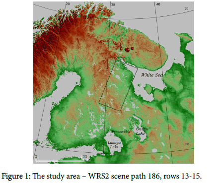
The area encompasses about 10 million ha in north taiga of Eastern Fennoscandia (Figure 1).
The altitude ranges from 0 to 350 m and the mean annual temperature is about 0°C, long-term mean annual precipitation is 500-550 mm. The area is a typical sample of continental glaciation. The Quaternary cover is formed by the glacial (moraine) and fluvioglacial (delta, sandur) deposits that cover Precambrian bedrock of the Fennoscandian Shield. They are locally overlain by lacustrine and marine sand-clay material and peat deposits. The exposures of ancient crystalline rocks are very common in denudation-tectonic relief prevailing here. The lake surface/drainage area ratio is remarkably high, 12% [10].
The area includes all main north taiga ecosystem types. There are three forest forming species here: Scots pine (Pinus silvestris L.), Finnish spruce (Picea x fennica (Regel) Kom.), and white birch (Betula pubescens Ehrh.). Due to intensive cuttings since the early 1960s, more than two-thirds of forests are currently younger than 50-60 years. The large fragments of old growth forests have remained only along the Finnish-Russian border.
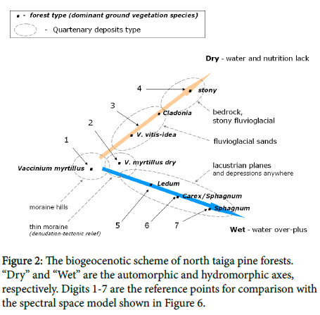
More than 80% of the forest land is covered with pine forests that occur in almost all types of habitats, formed on different Quaternary deposits [11]. Their diversity can be represented in the axes of the edaphic coordinates diverging from the ecological optimum (Figure 2).
Spruce-dominated stands (12% of the forest land) occur mostly on the slopes of moraine hills and wet depressions. Birch is an accompanying species in stand composition.
Due to excessive moistening and little evaporation, open mires occupy about one-third of the area. The largest mire systems are located on sea and lacustrine plains. Significant parts of forests are the ecotones between open mires and terrestrial ecosystems. The area is sparsely populated, with only one industrial center there – Kostomuksha ore-dressing mill. Agricultural lands (mostly meadows) occupy about 1.5%.
Image data and processing
Landsat ETM+ images from path 186 rows 13-14 acquired 2000.07.28 and row 15 (2002.06.16) were used for model creation. Landsat TM images from the same path, row 14 (1992.06.12) and row 15 (1990.06.23) were taken as time series, all obtained at ftp: //ftp.glcf.umd.edu/glcf/Landsat/WRS2
Localization of spectral classes within the model space was made using forest inventory maps, aerial photo and high resolution scanner images, landscape transects [11], and other ground data. Free RS/GIS packages QGIS, GRASS, SAGA were used for image processing; the gnuplot plotting utility was used for 3D visualization and analyzing the spectral space model.
Spectral space transformation
For the three-dimensional visualization of the spectral space, the axes of the classical Tasseled Cap transformation [12,13] can be used. Tasseled Cap is a linear transformation; therefore the lightest categories (cuttings, mires) occupy a large place in spectral space not due to their heterogeneity, but only to the largest value of albedo. Therefore, an attempt was made to use the logarithmic form of the original image values. As a result, an empirical transformation was obtained [8]. It reduces space to three axes LC1, LC2 and MSI: the two first principal components of the image matrix in logarithmic form, and Moisture Stress Index (SWIR1/NIR ratio). LC1 accounts for general scene brightness, LC2 correlates with quantity of green biomass, but not orthogonal to brightness. Three minimally mutually correlating bands were used for the axes LC calculation:
LC1 = 0.2793 × ln(R) + 0.7786 × ln(NIR) + 0.5619 × ln(SWIR2)
LC2 = 0.5887 × ln(R) – 0.6012 × ln(NIR) + 0.5404 × ln(SWIR2)
MSI = SWIR1/NIR
Where R, NIR, SWIR1, SWIR2- Landsat ETM+ bands 3, 4, 5, 7 digital numbers, respectively and ln- natural logarithm.
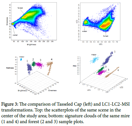
The logarithmic form equalizes to some extent the values of the dark forest and bright non-forest categories, with open water zone being scattered (Figure 3, top).
However, in the part of the space where forest and mire ecosystems are located the space becomes more “compact”, understandable, and suitable for analyzing (Figure 3, bottom). Even more importantly, the organizations of space are described here by simpler mathematical equations.
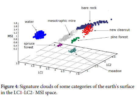
MSI is opposite to “wetness” and it makes space visually closer to human perception: dry and poor vegetation is at the hill top, rich and wet in the valley. The general organization of the space is shown in Figure 4.
Spectral space segmentation
Any of more or less homogeneous categories of an ecosystem (e.g., even-aged stand forest canopy or meadow surface) is represented in the model as an ellipsoid tilted to the plane of LC1-LC2 (Figure 4).
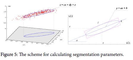
To determine the position and size of an ellipsoidal segment of each category, the point cloud is projected onto the plane LC1-LC2 (x and y, respectively), and the direction of the main axis of the ellipse is calculated from the regression line y = ax + b (Figure 5, right).
The dimensions of the ellipse (l and h) are determined as the coordinates of the most remote from the center points in the coordinate system, whose abscissa axis is parallel to the regression line. The position of the central plane of the ellipsoid in dimension MSI (z) is calculated from the regression equation from two variables z = cx + dy + e (Figure 5, left). All the segmentation parameters are given in Table 1.
| The position of the ellipse in the projection onto the x-y plane | The position of the ellipsoid central plane in dimension z | ||||||
|---|---|---|---|---|---|---|---|
| Coordinates of the center | Direction of the main axis* | Axes size | The coefficients of the regression equation z=cx+dy+e | ||||
| 1 | 2 | 3 | 4 | 5 | 6 | 7 | 8 |
| x | y | a | l | h | c | d | e |
Table 1: The parameters determining the position of the ellipsoid in the space LC1-LC2-MSI (x-y-z), Note: * - coefficient a in the equation of the regression line y = ax + b.
Thus, with this segmentation method, the shape of the category, its dimensions and position in space are accurately recorded. In traditional methods, only the coordinates of the center of the category and its overall dimensions are specified, while the shape is assumed as some invisible parallelepiped (in the method of the same name) or sphere (in minimum distance classification or MLC).
The simplest way to transform the spectral space model into the map is to set several points (for example, as a regular network) with the same category value inside each ellipsoid and then to use its LC1-LC2- MSI coordinates as class centers for the minimum distance classification. For implementation this algorithm, a special software module has been developed. Its input is LC1-LC2-MSI text file (red points cloud in (Figure 5); outputs are text files containing:
Array of 3D coordinates of ellipse blue line in (Figure 5)
Eight parameters (Table 1, bottom string)
Points for image classification. Point clouds for each category can be obtained, e.g. using GRASS module.
Results
The most essential features of the 3D spectral space model are described below step by step: a) mature and old growth forests: b) pine forest regeneration after cutting; c) open mires, and d) destroyed categories, starting with forest ecosystems located in the central, “core” part of spectral space. These categories include the vast majority of vegetation types of the territory, more than 95% of the area. For illustration purposes, only the centers of ellipsoid segments of ecosystem classes forming “molecule” ball-and-stick chains are shown.
Mature and old growth forests
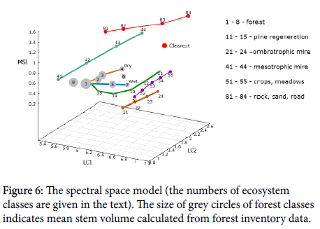
The biogeocenotic scheme shown in Figure 2 is an “imaginary” construction, based on ground observations, while the spectral space model is real, albeit virtual. Nevertheless, the location of reference points 1-7 in Figure 2 almost completely coincides with the position of the mature and old-growth pine forest classes in spectral space (Figure 6).
Both gradient lines, dry and wet, go along axis LC1 from dark to bright parts of spectral space due to reduction of radiation absorption by canopy caused by decreasing leaf area index (LAI), which, in turn, is a result of edaphic conditions deterioration. Besides, along the dry gradient the moisture stress grows, and line goes up. There is no moisture lack along the wet gradient, and the line remains almost horizontal. Due to their wide ecological amplitude, pine stands occupy all the forest zone of spectral space. Class 1 is the most productive mixed pine-spruce-birch forest with spruce undergrowth. Dominant ground vegetation species are Vaccinium myrtillus and V. vitis-idaea; the soils are Ferric and Ferric-Carbic Podzol. Class 3 is pure pine stands on fluvioglacial sands, with pine undergrowth; the soil is sandy shallow Podzol. Wet concave spots are of the V. vitis-idaea type, while dry convex ones are of the Cladonia type. Class 4 represents low productive pine stands growing on bedrock or boulder fluvioglacial sediments with primitive soils (Leptosol). The ecosystems located along the wet gradient line are the ecotones between automorphic habitats and open mires. Class 5 is formed by mixed pine-birch-spruce stands at an intermediate stage of paludifcation with a thin peat layer (up to 0.3-0.5 m); the ground vegetation is a dwarf shrub (Ledum palustre, Vaccinium uliginosum). Classes 6 and 7 are sparse pine stands of Sphagnum and Carex-Sphagnum type, respectively.
Classes 5 and 6 occupy large areas at the periphery of mesotrophic mires; class 7 is commonly a narrow strip alone the edge of ombrotrophic mires. The strip width is often less than 30 m, so the scanner is unable to register it. Thus, in most cases, the location of pine forests in spectral space coincides with their location in the axis of edaphic and phytocenotic coordinates, and the biogeocenotic complexes (Quaternary deposits + vegetation) can be identified. Obviously, the scanner registers not the type of Quaternary sediments as such, but the conditions of water and mineral nutrition, most typical for specific type of habitats.
Class 2 is relatively ambiguous, it can be considered as the upper right part of class 1 ellipsoid segment. Its "content" can be denoted as the “open canopy conifer stands”. Due to pixel size 30x30 m, the scanner registers mixed signal from crowns, ground vegetation, and tree shadows, which makes it impossible to determine the tree species composition, and even dominant species. In some cases, this is possible by using the landscape context; e.g., in denudation-tectonic relief, this class includes pine-dominated or mixed pine-spruce stands of the dry myrtillus type, while on abraded, smoothed drumlins of sea plane (the White Sea lowland) one can find spruce stands of the wet myrtillus type. If a sufficiently detailed digital elevation model (DEM) existed, then the discrimination of these classes could have been made with the use of some geomorphometric indexes [14]. Thus, the two types of habitats above have rather different values of fractal dimension. It should be noted that these classes are rather similar types of vegetation in terms of the mass and energy exchange (without account of tree species composition).
Class 8 is represented by spruce-dominated stands with closed canopy growing on the slopes of moraine hills (myrtillus type), and more wet variants (Sphagnum/myrtillus) occupying gentle slopes at the foot of hills and depressions. Stands of this type have high LAI; most solar energy is absorbed, making them difficult targets for discrimination of classes. Thus, class 2 is ambiguous due to low canopy density, while class 8- owing to high density. In both cases discrimination is possible using DEM.
A more or less significant proportion of spruce in stand composition is observed in classes 1, 2, and 5, closest to the optimal edaphic condition. In these classes, the share of birch may reach 20-30%. All forest classes have a few parts with different canopy density, so the total number of mature forest categories exceeds 20.
Pine regeneration
The cutting in this territory is carried out in the most productive habitats (classes 1 and 3 in Figure 6). The locations of new clearcut class are almost the same for both habitats, but the succession trajectories of forest regeneration through spectral space are sharply different depending on the type of Quaternary deposits. In Figure 6 the regeneration trajectory on the moraine is shown: 11 – first vegetation appearance; 12-13 – young; 14 – middle age; 15 – ripening stands. On fluvioglacial sands, where the regeneration goes without the participation of birch and aspen, the trajectory is almost a straight line from clearcut to class 3, and age stages are less distinguishable than on the moraine. Multi-temporal images are required for better discrimination.
The exact position of the trajectory end point (pine or spruce domination), as well as succession velocity, especially at last stages, depends on local conditions: landscape context, details of edaphic features, and the availability of spruce and/or pine seeds.
Open mires in this territory are presented by two main types of water and mineral nutrition: ombrotrophic (classes 21-24) and mesotrophic (classes 41-44). These mires have significantly different microrelief and vegetation cover; dominant species are Sphagnum and Carex, respectively. Due to differences in spectral response curve, in spectral space mires encircle the forest zone from opposite sides.
Different types of mires form long ellipsoids of complex shape; only the main centerlines are shown here. Position in spectral space along the LC1 axes reflects the level of water table, from inner lakes and pools in the dark part of space (classes 21 and 41) to the dried plots (classes 24 and 44) occupying the brightest part.
Deeply transformed ecosystems (shrubs, meadows, crops) are located in the right, lightest part of space (classes 51-55). Nonvegetation categories, such as sands, roads and settlements (classes 81-84), occupy the zone with the maximum LC2 and MSI value.
Ecosystem map
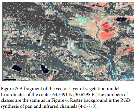
The vectorized classification result of image classification using 3D spectral space model is shown in Figure 7.
Two-step generalization was applied: “mode” filtering to the classified raster and the cleaning topology tool “remove small areas” after vectorization.
Ecosystem characteristics
The position in spectral space defines a type of the biogeocenoic complex (Quaternary deposits + vegetation), which, in turn, determines the net ecosystem production, carbon pool, soil type, tree species composition, ground vegetation, i.e. qualitative, intrinsic biogeocenotic characteristics. Specific quantitative values of such parameters as stand characteristics (stem volume, average height and diameter, etc.), can be calculated using forest inventory data. These values compose the attribute data of the vector layer. So, the ecosystem map can produce a set of very different thematic maps: land use categories, Quaternary deposits, forest inventory, soil and mire types, biological productivity, anthropogenic disturbance, etc.
Mathematical model of the spectral space trajectories
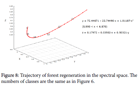
The model of the spectral space makes it possible to describe the trajectories of types of habitats as well as different succession stages mathematically. As an example the line of pine regeneration is shown in Figure 8.
The line in 3D space is described by a system of two equations:
y=f1(x);
z=f2(x, y);
Where x, y, z- LC1, LC2, MSI and f1, f2- polynomial regression of 1st -3rd degree.
The principle of trajectory description is the same as for ellipsoids enveloping curve: the first equation describes the line of the trajectory projection on the LC1-LC2 plane, the second - the position of the trajectory in the third dimension (MSI). These equations can be used as transfer functions for calculating various ecosystem parameters. In this case it can be, for example, the age-biomass curve.
Discussion
Figure 6 shows that spectral space of the Landsat image is a complicated system of ellipsoids and trajectories. However, it can be quite easily interpreted in ecological terms. The investigation of these patterns to create a ecosystem map is thought to be much more reasonable, effective, and interesting than “blind” supervised classification. The process starts with the biogeocenotic scheme creation (Figure 2) by studying available materials on vegetation types and Quaternary deposits of the study area. At this stage, the visible scanner image of the area is created (RGB-synthesis from infrared channels). This is much more informative than the unsupervised classification traditionally used on this case.
As a result of the analysis of all the data, the first variant of the classification scheme is obtained. The next step is to build the spectral space model. Protected areas are believed to be ideal as reference objects because their ecosystems are undisturbed (this facilitates the localization of spectral classes) and usually well studied and mapped.
After preliminary localization of the main ecosystem classes in spectral space and its visualization, the model refinement begins and the advantages of 3D modeling become apparent. The capability to examine the whole spectral space from any side, as well as the location and relative position of different categories are fundamentally important as it involves human intuition into analysis.
The spectral space model makes it possible to purposefully correct the position of class centers in space by editing the statistical table for the minimum distance classification and to find optimal classification variant by the trial-and-error method. The supervised classification is one-directional, i.e. it goes from training sites to the entire image. In 3D space, interpolation becomes possible. It is logical to assume that the categories with intermediate characteristics can be found in the space span between classes with known properties. To test this hypothesis we can simply add a new line with space coordinates into the statistical table for classification. We can also determine where the category occupying a specific part of spectral space is located in the map. And, most importantly, there is the possibility to see the classification results both in geographical and spectral space, e.g. as a set of points clouds. To conclude, the classification can be transformed from supervised to manageable one, thus allowing extracting a greater amount of information from the image.
Segmentation of the spectral space by the method of ellipsoids provides more accurate, in comparison with traditional methods, the delineation of the spatial configuration of the ecosystem contours. This is fundamentally important for change detection on the time series images, and also for the most accurate matching of the vegetation cover model with DEM in hydrological modeling.
These new opportunities improve our understanding of the way the scanner recognizes different types of vegetation, and provide a much more effective feedback mechanism of training sites selection, as compared to the accuracy assessment by the kappa statistics. In some cases, classes’ discrimination by non-visual methods is practically impossible, but is very simple in visible 3D space. This can be applied to forest edges at the borders with mires and lakes, as well as to any types of narrow ecotones. Preliminary results have shown that the proportion of such categories in the study area is remarkably high.
The spectral space model is a link between technical image information and human understanding of ecosystems typology. It plays the role of interactive, mobile classification scheme. Creating the spectral space model is a long-term research process. As a result, the first detailed digital map of the biogeocenotic structure for the study area has been compiled. The model includes all basic classes of primary ecosystems, and some variants and stages of their natural and anthropogenic disturbances. The number of detail is constantly increasing. Accuracy assessment was carried out by comparing with the georeferenced database “CORINE-biotopes” [15]. Taking into account the level of generalization, the degree of identity was almost 100% [16]. Such accuracy is quite explicable. Plants and environment are interacting as a physico-chemical system [17]. The scanner registers the physical characteristics of biogeocenosis. This allows allocating a relatively small number of generalized ecosystem classes with an almost absolute certainty. Decomposition of the spectral classes using DEM and time-series images could increase the total number of recognized classes of vegetation several times. It should be noted that currently the main barrier to increase the map detail is the lack of high resolution DEM. The ideal variant would be the use of LiDAR data, which would also allow receiving the information on canopy architecture.
Conclusion
The ecosystem-biophysical approach to the processing of scanner images is the integration of two arrays of information: a) graphically expressed idea of the biogeocenotic structure of the territory formed as a result of ground-based research, and b) a three-dimensional model of the spectral space created on the basis of the biophysical characteristics of ecosystems measured by the scanner. It includes three key components: creation of graphical expression of forest and mire cover typology (biogeocenotic scheme); transformation of image spectral space into a visible 3D form; and comparison of the positions of the ecosystem signatures in spectral space with the biogecenotic scheme.
The spectral space model reflects the continual structure and dynamics of vegetation cover in space and time in a clearly visible form. The model analysis substantially facilitates the classification process and allows extracting much more information from the image than in the tradition approach, in which the characteristics of vegetation cover are identified by means of their correlation with signal levels in different scanner bands. The proposed approach implies the identification of types of ecosystems through their position in the spectral space of the image. The decomposition of spectral classes is carried out with the use of DEM, this significantly increases the reliability of the final result. The complex characteristics of vegetation are defined as inherent in the particular types of biogeocenoses.
The spectral space model is a mathematically formalized object which integrates discrete field observations data into the continuum describing the quantitative and qualitative characteristics of the ecosystems. Being deployed in geographical space, it turns into the optimal structural base for integrating the results of discrete field observations into a single space-time continuum.
Spatial information derived from spectral space models can be useful for a variety of scientific and practical purposes: forest management and the monitoring of landscape mosaic dynamics on the regional level; estimation of carbon balance components etc. However, its mission seems to be more fundamental. Perhaps, the spectral space model can serve as the foundation for objective classification of ecosystems, where one of the most significant clustering criteria is the mathematically expressed position in spectral space. Practically, it will help reduce uncertainty in forest mapping at the global level. The biophysical base of such a classification makes it independent of local (forestry, geobotanical) typologies and, thus, provides an opportunity for creating an internally consistent vegetation map for large areas.
The development of the model goes in increasing the accuracy and detailing, and expanding the territory. At present, the model of the Onega Lake and the White Sea catchment area is being carried out. In particular, these models are used to estimate the intake of dissolved organic carbon.
In practical sense, the described technique is most useful to those researchers who are not satisfied with the quality of information obtained from images by traditional methods. Preliminary analysis has shown that spectral models are rather similar in TM/ETM+ images of Fennoscandia, Siberia and Canada. It would be beneficial to test this approach in similar natural conditions. In our opinion, it is likely to be of interest to the unconventionally minded researchers and students.
Acknowledgement
The work was carried out within the framework of the State task of the Northern Water Problems Institute KarRC RAS.
References
- Tomppo E, Czaplewsk, RL (2002) Potential for a remote sensing-aided forest resource survey for the whole globe. Unasylva 53: 16-18.
- Pekkarinen A, Reithmaier L, Strobl P (2009) Pan-European forest/nonforest mapping with landsat ETM+ and CORINE land cover 2000 data. J Photogramm Remote Sens 64: 171-183.
- Hirata Y, Takahashi T (2011) Image segmentation and classification of landsat thematic mapper data using a sampling approach for forest cover assessment. Can J For Res 41: 35-43.
- Kanellopoulos I, Wilkinson GG, (1997) Strategies and best practice for neural network image classification. Int J Remote Sens 18: 711-725.
- Zhou L, Yang X (2008) Use of neural networks for land cover classification from remotely sensed imagery. ISPRS 37: 575-578.
- Litinsky P (1997) Assessment of forest decline around Kostomuksha ore-dressing mill using satellite images. In: Ecosystems, fauna and flora of the Finnish-Russian Nature Reserve Friendship. Finnish Environment Institute, Helsinki, Finland, pp. 341-346.
- Litinsky P (2007) 3D modeling of taiga landscapes structure and dynamics, KarRC RAS, Petrozavodsk, Russia.
- Litinsky P (2011) Multispectral imagery classification method based on spectral space modeling. Transactions of KarRC RAS 2011: 45-54.
- Litinsky P (2012) Geoinformation model of Eastern Fennoscandia Northern Taiga ecosystems. Transactions of KarRC RAS 2012: 3-15.
- Antikvaari, Biotic diversity of Karelia: Conditions of formation, communities and species (2003) KarRC RAS, Petrozavodsk, Russia.
- Volkov AD, Gromtzev AN, Erukov GV (1995) Ecosystems of north-west taiga landscapes (structure, dynamics). Petrozavodsk: KarRC RAS 1995: 194.
- Kauth RJ, Thomas GS (1976) The Tasseled Cap a graphic description of the spectral-temporal development of agricultural crops as seen by Landsat. In: Proceedings on the Symposium on Machine Processing of Remotely Sensed Data, Purdue University, West Lafayette, Indiana.
- Huang C, Yang WL, Homer C, Zylstra G (2002) Derivation of a tasselled cap transformation based on landsat 7 at-satellite reflectance. Int J Remote Sens 23: 1741-1748.
- Wood J (1996) The geomorphological characterization of digital elevation models. Department of Geography, University of Leicester, England, UK.
- Söderman T (1997) Biotopes Mapping of the Eastern Baltic. CORINE Biotopes 17 Project in the Baltic States and Northwestern Russia. Nord, Russia.
- Kryshen A, Litinsky P (2013) Comparison and mutual verification of the geoinformation and the ecological dynamics models of forest ecosystems diversity. Transactions of KarRC RAS 2013: 86-91.
- Pignatti S, Box EO, Fujiwara K (2002) A new paradigm for the XXIth century. Ann Bot 2: 3057.
 Spanish
  Chinese
  Russian
  German
  French
  Japanese
  Portuguese
  Hindi
Hindi 