Spanish
  Chinese
  Russian
  German
  French
  Japanese
  Portuguese
  Hindi
Hindi Short Communication, Geoinfor Geostat An Overview Vol: 9 Issue: 1
WEB MAPPING ERA IN GEOINFORMATICS
Bruce T. T. Calvert*
Independent Researcher, Ottawa, Canada
*Correspondence:
Niharika Dvivedi
Independent Researcher
Ottawa, Canada
E-mail: brucetcalvert@gmail.com
Received: December 09, 2020 Accepted: January 21, 2021 Published: January 28, 2021
Citation: Calvert BTT (2020) Correcting for Amplification Bias and Sea Ice Bias in Global Temperature Datasets. Geoinfor Geostat: An Overview 9:1.
Abstract
Web mapping and therefore the geospatial information online has evolved rapidly over the past few decades round the world. Almost every mobile now has location services and each event and object on the world features a location. the utilization of this geospatial location data has expanded rapidly, because of the event of the web. Huge volumes of geospatial data are available and daily being captured online, and are utilized in web applications and maps for viewing, analysis, modelling and simulation. This paper reviews the developments of web mapping from the primary static online map images to the present highly interactive, multisourced web mapping services that are increasingly moved to cloud computing platforms. the entire environment of web mapping captures the mixing and interaction between three components found online, namely, geospatial information, people and functionality. during this paper, the trends and interactions among these components are identified and reviewed in reference to the technology developments.
Keywords: Climate Change; Global Warming; Instrumental; Temperature; Amplification; Sea Ice; Bias; Maximum Likelihood; Internal Variability; El Niño
Keywords
Climate Change; Global Warming; Instrumental; Temperature; Amplification; Sea Ice; Bias; Maximum Likelihood; Internal Variability; El Niño
Introduction
Estimating the evolution of global surface temperatures since the industrial revolution is important as it can help improve understanding of the Earth’s climate system. Currently, there are various GITDs, including HadCRUT4 [1] by the UK Met Office Hadley Centre (Met Office) in conjunction with the Climatic Research Unit (CRU) of the University of East Anglia, GISTEMPv4 [2] by NASA’s Goddard Institute of Space Studies, and NOAAGlobalTempv5 [3-5] by NOAA’s National Climate Data Centre. One major issue with estimating past temperatures is that not all regions of the Earth have complete observational records. As a result, one must statistically infer temperatures of unobserved regions of the planet using available data to properly understand the evolution of global surface temperatures since the industrial revolution.
In the past decade, two new GITDs have been created that use a geostatistical technique known as kriging [6,7] to infill temperatures for unobserved regions of the Earth: Berkeley Earth Surface Temperature [8-10], and Cowtan and Way [11,12]. For convenience, this paper refers to Berkeley Earth Surface Temperature using LSATs for sea ice regions as BEST, and refers to the long reconstructions of Cowtan and Way version 2 using HadSST3 [13,14] and HadSST4 [15] as C&W-HadSST3 and C&W respectively. Kriging has desirable statistical properties: if covariances between temperature observations are known with certainty, then kriging provides the most-efficient linear unbiased estimates of temperatures of unobserved regions. In addition, the kriging estimates are identical to the maximum likelihood estimates if the distribution of residuals is multivariate normal.
While kriging has desirable statistical properties when covariances between temperature observations are known with certainty, in reality, these covariances are unknown and must be empirically estimated from available data. Ordinary kriging, by itself, does not provide a method to empirically estimate these covariances, nor does it account for the uncertainty due to estimating these covariances. To address these issues, this study uses MLE to estimate parameters in the covariance function and quantify their uncertainty. MLE has very desirable statistical properties when the number of observations is large: consistency, asymptotic efficiency, and asymptotic normality.
The underlying statistical models of BEST and C&W do not adequately account for the statistical tendency of different regions of the planet to warm at different rates and, therefore, are subject to amplification bias. In addition, C&W does not account for changes in sea ice and so is subject to sea ice bias. To quantify these biases, the Akaike information criterion (AIC) [16] was used to select the best of 16 different temperature anomaly models and the best of 24 different temperature climatology models. Using AIC to pick from a large set of models helps reduce omitted variable bias and avoid the statistical issue of overfitting. The best models were combined to construct a new GITD. This GITD is given the name HadCRU_MLE, to reflect its use of MLE and data primarily from the Met Office and CRU. Similar to C&W, LSAT anomalies of HadCRUT4 and SST anomalies of HadSST4 were used, so the results of this study are most comparable to the results of C&W.
Data
5° by 5° gridded monthly temperature anomalies of HadCRUT4 and HadSST3 were obtained from the Met Office website. This includes 100 ensemble members as well as ensemble medians. These datasets were used to infer LSAT anomalies of HadCRUT4, which are essentially CRUTEM4 [17] but with adjustments to account for biases and uncertainties such as due to temperature homogenization and the urban heat island effect. Measurement and sampling uncertainties of CRUTEM4 were also obtained.
5° by 5° gridded monthly temperature anomalies of HadSST4 were obtained from the Met Office website. This includes 200 ensemble members, which account for bias uncertainties, as well as the ensemble median. The 100 ensemble members of HadCRUT4 LSAT anomalies were combined with the 200 ensemble members of HadSST4 to produce 200 ensemble members of temperature anomaly observations; each LSAT ensemble member was used twice. Error covariance matrices and total uncertainty of HadSST4, which account for measurement and sampling uncertainties, were also obtained.
0.25° by 0.25° gridded land mask data of OSTIA [18] was obtained from the Copernicus Marine Environment Monitoring Service website. OSTIA data was integrated to a 5° by 5° grid to replicate the land fraction data used in HadCRUT4. OSTIA data was also integrated to a 1° by 1° grid. OSTIA was used in combination with the HadCRUT4, HadSST3, and CRUTEM4 data to infer LSAT anomalies of HadCRUT4.
1° by 1° gridded monthly sea ice concentrations (SICs) of HadISST1 [19] and HadISST2 [20] were obtained from the Met Office website. These SICs were component-wise multiplied by the non-land fraction to obtain sea ice fractions (SIFs). This paper defines the SIF of a grid cell as the fraction of the total surface area of a grid cell covered by sea ice. SIFs were integrated to a 5° by 5° grid. HadISST2 was used as the main SIC dataset of this study; HadISST1 was used only to determine how much sea ice extent varies between datasets.
The 5° by 5° gridded 1961-1990 temperature climatology of Jones et al. [21] and 100 ensemble members of the 5° by 5° gridded 1961- 1990 temperature climatology of HadSST3 were obtained from the Met Office website. These temperature climatologies were used to help estimate and correct for sea ice bias. The 1° by 1° gridded 1979-1998 temperature climatology of IABP-POLES [22] was obtained from the University of Washington website. IABP-POLES were used to test for the impact of spatial resolution on the estimate of sea ice bias.Time series data of the ensemble medians of C&W-HadSST3 and C&W was obtained from the University of York website. In addition, time series data of BEST was obtained from the Berkeley Earth website. These datasets were used for comparison with the results of this study.
30 arc-second resolution GMTED2010 surface elevation data [23] was obtained from the US Geological Survey website. This was integrated to a 0.25° by 0.25° grid. This was combined with the land fraction data and integrated to a 5° by 5° grid to produce average surface elevation data for land regions and non-land regions. This average surface elevation data was used to help explain variation in the temperature climatology.
CCSM4 output for the pre-industrial control scenario and for the RCP6.0 scenario was obtained from the University Corporation of Atmospheric Research website. This includes monthly gridded surface air temperatures (SATs) 2 m above the surface and monthly gridded SICs. The climate model output for the pre-industrial control scenario was used to estimate temperature patterns of internal variability. As the RCP6.0 scenario roughly corresponds to historic forcing, the output for the RCP6.0 scenario was used for comparison with the corrections for sea ice bias of this study. CCSM4 was chosen because it “has been analysed the most extensively of any current climate model with regards to [interdecadal Pacific variability] processes and mechanisms, and compares favourably in those aspects to observations” [24]. Only the last 501 years (800-1300) of the pre-industrial control scenario were used because the model was not necessarily in equilibrium at the beginning of the model run.
SICs of CCSM4 are given in a Greenland pole grid, where the North Pole is moved to Greenland to avoid singularity problems in the sea ice model. Nearest neighbour interpolation was performed to convert SICs to a 0.125° by 0.125° grid; this small grid size was used to reduce interpolation error. These SICs were integrated to a 0.25° by 0.25° grid and component-wise multiplied by the non-land fraction to obtain SIFs. Similarly, SATs, which are given in a 1.25° longitude by 0.9375° latitude grid, were converted to a 0.125° by 0.125° grid using nearest neighbour interpolation. SIFs and SATs were integrated to a 5° by 5° grid. 5° by 5° climatologies of SIFs and SATs for the preindustrial control scenario were constructed by taking averages by calendar month.
Monthly Southern Oscillation Index (SOI) [25] data was obtained from the Australian Government website. The SOI is based upon the pressure difference between Darwin, Australia and Tahiti, and is strongly correlated with ENSO. This index was compared with the estimated ENSO behaviour of this study.
The versions of the datasets used in this study were their most upto- date versions at the time of download. Data after December 2018 was not used as HadSST4 data after December 2018 was not available at the time of download. Results of this study are often given as the change from the late 1800s to 2018; the entire late 1800s is used as uncertainties of annual GMST anomalies in the late 1800s are large and 2018 is used as it is the most recent year with data for all calendar months.
Methods
Amplification bias
Adopting the notation of Berkeley Earth, the temperature  at a
position on the Earth’s surface
at a
position on the Earth’s surface  and time in months t is

where mt is the calendar month of t,  is the temperature
climatology at for calendar month mt, θt is a constant for month t,
and W is a weather residual term.
is the temperature
climatology at for calendar month mt, θt is a constant for month t,
and W is a weather residual term.
For this paper, θ can differ from the GMST and is replaced with
( , s) , where corresponds to the mid latitude and mid longitude of
a 5° by 5° grid cell, and S is the surface type; s=0 for open sea (referred
to as sea) and s=1 for land or sea ice (referred to as land-ice). For
convenience, is called a grid cell and (, s) is called a grid subcell.
This study adopts the convention of GISTEMP, BEST, and C&W of
treating SATs above sea ice similarly to LSATs since SATs above sea ice
tend to more closely resemble LSATs than SATs above sea (also called
marine air temperatures (MATs)). Thus, (1) becomes

Similar to C&W, C is taken to be the 1961-1990 temperature climatology. Thus, (2) simplifies to become

where  is the local temperature anomaly at ( , s) for month t.
In reality, observations of temperature anomalies are subject to measurement, sampling, and bias uncertainties. Thus, (3) is modified to become

where  is the temperature anomaly observation at (x s) for
month t and
is the temperature anomaly observation at (x s) for
month t and  is the error due to measurement, sampling, and bias uncertainties at ( , s)
for month t.
is the error due to measurement, sampling, and bias uncertainties at ( , s)
for month t.
Equation (4) implicitly assumes that all regions of the Earth have a statistical tendency to warm at the same rate. However, polar regions tend to warm faster due to the snow-albedo feedback and because global warming increases heat transfer from equatorial regions to polar regions. This increased heat transfer occurs partly because warmer air can hold more water vapour and thus can have a higher heat capacity. In addition, sea regions tend to warm more slowly than land regions, as water has a higher heat capacity than land. As a result, the assumption that all regions have a statistical tendency to warm at the same rate can lead to amplification bias. When amplification bias is ignored, unobserved regions are infilled with temperature anomalies that are biased towards the GMST anomaly. Since polar regions such as Antarctica, the Southern Ocean, and the Arctic Ocean were poorly observed during the instrumental period, not accounting for amplification bias should cause an underestimation of the rate of GMST change as these regions tend to have high local amplification factors (LAFs).
To try to correct for amplification bias, (4) is modified to become

where  is called the LAF at ( , s)
for calendar month m and
is defined to have a surface area weighted mean of one over the
Earth’s surface for each calendar month (assuming that SICs are
the 1961-1990 HadISST2 mean by calendar month). In reality, the
amplification function A could change from one year to the next.
However, modelling studies find that the assumption of unchanging
LAFs over the instrumental period is reasonable [26,27] and find that
LAFs are mostly independent of the type of climate driver [28]. This
suggests that (5) should correct for most amplification bias.
is called the LAF at ( , s)
for calendar month m and
is defined to have a surface area weighted mean of one over the
Earth’s surface for each calendar month (assuming that SICs are
the 1961-1990 HadISST2 mean by calendar month). In reality, the
amplification function A could change from one year to the next.
However, modelling studies find that the assumption of unchanging
LAFs over the instrumental period is reasonable [26,27] and find that
LAFs are mostly independent of the type of climate driver [28]. This
suggests that (5) should correct for most amplification bias.
This study tested four different functional forms of the amplification function (Table 1) to determine if LAFs are affected by calendar month, latitude, or surface type. For simplicity, the impact of latitude on A was treated as a polynomial of order at most four. In addition, the derivative of A with respect to latitude was restricted to zero at the poles to ensure smoothness at the poles. All four functional forms can be expressed as

Table 1: The different models of the amplification function. These models were used to estimate temperature anomalies.
| Model | Amplification function depends on latitude? | Amplification function depends on surface type? | Amplification function depends on calendar month? |
|---|---|---|---|
| 1 | No | No | No |
| 2 | No | Yes | Yes |
| 3 | Polynomial of order four | No | Yes |
| 4 | Polynomial of order four | Yes | Yes |
where  and F has a surface area
weighted mean of zero for each calendar month.
and F has a surface area
weighted mean of zero for each calendar month.
Internal variability, such as from ENSO, may cause issues in estimating A. Polar regions tend to warm faster than equatorial regions. However, an El Niño event causes significant short term warming that is concentrated in equatorial regions, particularly in the Eastern Equatorial Pacific Ocean. As a result, if one estimates A using (5) and (6), then ENSO could bias the estimate of A towards the identity function.
To try to avoid this ENSO bias and allow for internal variability to be incorporated into the model, (5) is modified to become

where  is the number of internal variability patterns (IVPs) in the model, qt,I is an index for month t that
corresponds to the
is the number of internal variability patterns (IVPs) in the model, qt,I is an index for month t that
corresponds to the  and
and  is the value of the ith IVP at . One IVP was obtained (see later
subsection on IVPs), corresponding to ENSO, and this study tested
models that contain zero or one IVPs. While only one IVP was used,
the statistical framework of this study can be easily extended to
incorporate more IVPs.
is the value of the ith IVP at . One IVP was obtained (see later
subsection on IVPs), corresponding to ENSO, and this study tested
models that contain zero or one IVPs. While only one IVP was used,
the statistical framework of this study can be easily extended to
incorporate more IVPs.
To estimate model parameters in (7) using MLE, a model of W is needed. W is assumed to be multivariate normal with a mean of zero and with covariance function
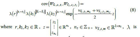
the standard logistic function, an  is the great circle distance
between
is the great circle distance
between  In this model, r determines the temporal
autocorrelation of weather residuals, k1 determines the spatial
correlation of weather residuals, k2 affects the correlation between
land-ice and sea weather residuals, and z determines the variances.
The standard logistic function constrains temporal and spatial
correlations between zero and one, which ensures physically sensible
results and improves numeric stability of the estimation procedure.
In this model, r determines the temporal
autocorrelation of weather residuals, k1 determines the spatial
correlation of weather residuals, k2 affects the correlation between
land-ice and sea weather residuals, and z determines the variances.
The standard logistic function constrains temporal and spatial
correlations between zero and one, which ensures physically sensible
results and improves numeric stability of the estimation procedure.
Two different models of the covariance function were tested (Table 2) to determine if the variance of weather residuals is affected by surface type. The models of the covariance function are simple compared to the models of the amplification function since additional parameters in the covariance function are more computationally intensive than additional parameters in the amplification function.
Table 2: The different models of the covariance function of weather residuals. These models were used to estimate temperature anomalies.
| Model | Covariance function depends on latitude? | Covariance function depends on surface type? | Covariance function depends on calendar month? |
|---|---|---|---|
| 1 | No | No | No |
| 2 | No | Yes | No |
GISTEMP, BEST, and C&W infill land-ice and sea regions separately as it were found to give better results. However, the introduction of the amplification function puts this practice into doubt. Perhaps this approach gave better results due to differences in LAFs between land-ice and sea regions. The statistical models tested in this study account for correlations between land-ice and sea weather residuals, which can improve temperature anomaly estimates.
Alternatively, perhaps infilling land-ice and sea regions separately gave better results due to differences in their correlation decay lengths. This paper defines the correlation decay length as the distance between two locations required reducing the spatial correlation of their residuals to e-1. However, C&W estimate similar correlation decay lengths for weather residuals: 767 km and 860 km for land-ice and sea regions respectively. Similarly, BEST has similar maximum correlation lengths: 3310 km and 2680 km for land-ice and sea regions respectively, corresponding to correlation decay lengths of 1497 km and 1212 km respectively. Having different correlation decay lengths for land-ice and sea regions was considered, but this approach was not taken due to its high computational cost. As C&W and BEST estimate similar correlation decay lengths for land-ice and sea regions, the impact of using identical correlation decay lengths for land-ice and sea regions should be minimal.
The four models of the amplification function were combined with the two models of the covariance function and using zero or one IVPs to produce 16 different temperature anomaly models. To estimate a temperature anomaly model, an iterative approach to MLE was taken, where a reasonable first guess was calculated and used in combination with a saddle-free Newton’s method [29,30]. To make the procedure computationally feasible, numeric approximations to the log-likelihood function were used and their derivations are given in the supplementary information. As the bias uncertainties of E have a complicated covariance structure, do not have a multivariate normal distribution, and have significant temporal correlation, numeric approximations that account for bias uncertainties could not be derived. As a result, bias uncertainties were neglected in the estimation of the temperature anomaly model. However, bias uncertainties were still taken into account in the estimation of total uncertainty.
The best of the 16 models was chosen by minimizing the AIC. To reduce computation time, only six of the 16 models were estimated and the best temperature anomaly model was chosen in a stepwise manner. Firstly, the best covariance function was chosen by estimating the two covariance functions with the first amplification function and zero IVPs and picking the model with the lowest AIC. Secondly, the best amplification function was chosen by estimating the best covariance function with the other three amplification functions and zero IVPs, and picking the model with the lowest AIC. Finally, the best covariance function was estimated with the best amplification function and the IVP for ENSO. For comparison, Bayesian information criterion (BIC) [31] values were also calculated. This paper presents normalized AIC and BIC values (nAIC and nBIC), which are normalized by the number of observations.
For each of the six models, maximum likelihood estimates of temperature anomalies were calculated for all combinations of grid subcells and months. Land-ice and sea temperature anomalies were then blended, by weighting observations using SICs of the 1961-1990 HadISST2 mean by calendar month. For the model with the lowest AIC, its uncertainty was evaluated using a Monte Carlo approach. The Monte Carlo approach produced 200 ensemble members of temperature anomalies, which account for measurement, sampling, model parameter, infilling, and bias uncertainties.
Sea Ice Bias
When sea ice is replaced with open sea, an increase in SATs is observed empirically [22] and in climate models [32,33]. This is because sea water has a lower albedo than sea ice and because sea ice acts as an insulator that prevents heat transfer between colder air and warmer water. As a result, not accounting for changes in sea ice can lead to sea ice bias. In particular, as warming has caused sea ice to melt, neglecting sea ice bias leads to an underestimation of GMST change over the instrumental period. C&W assumes constant SICs for each calendar month and uses the 1981-2010 HadISST1 median by calendar month. As a result, C&W may underestimate GMST change over the instrumental period. In comparison, BEST varies SICs according to HadISST2 and, partially as a result, shows more warming over the instrumental period than C&W.
To correct for sea ice bias, a temperature climatology model was combined with the best temperature anomaly model to estimate temperature differences between sea ice and open sea. The estimated temperature differences were used to estimate and correct for sea ice bias. Since HadSST4 and CRUTEM4 are temperature anomaly datasets, suitable temperature climatology datasets that correspond to these temperature anomaly datasets should be used to estimate a temperature climatology model. Since a temperature climatology for HadSST4 was not available, the HadSST3 climatology was used as the temperature climatology corresponding to HadSST4.
CRUTEM4 does not have a corresponding LSAT climatology. However, the Met Office website lists the 1961-1990 temperature climatology of Jones et al. along with its main temperature anomaly datasets of HadCRUT4, HadSST3, and CRUTEM4. The Jones et al. climatology was constructed using CRUCL1 [34] for land regions north of 60°S, IABP-POLES for sea ice regions north of 60°N, a combination of MAT and SST observations for sea regions north of 60°S, and LSAT observations of Antarctica for land regions south of 60°S.
Climatologies corresponding to CRUTEM4 were inferred from the Jones et al. climatology. The following model was used to explain variation in the temperature climatology

where  is the temperature climatology at for calendar month
  contains explanatory variables
at for calendar month m, and U is a term for the temperature
climatology residual. In particular,
contains explanatory variables
at for calendar month m, and U is a term for the temperature
climatology residual. In particular,  is given the functional
form
is given the functional
form
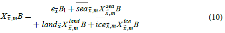
where  is the average surface elevation at , land is the fraction
of grid cell covered by land,
is the average surface elevation at , land is the fraction
of grid cell covered by land,  is the SIF of grid cell for
calendar month m using SICs of the 1961-1990 HadISST2 mean by calendar month,
is the SIF of grid cell for
calendar month m using SICs of the 1961-1990 HadISST2 mean by calendar month,  and X ice are defined implicitly.
 is assumed to be multivariate normal with a mean of zero and
with covariance function
is assumed to be multivariate normal with a mean of zero and
with covariance function
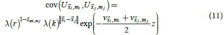
where  is the
Kronecker delta. In this model, r determines the temporal correlation
of residuals, k determines the spatial correlation of residuals, and z determines the variances. Variables in (8) are repeated in (11) for ease
of communication; however, temperature climatology models and
temperature anomaly models were estimated independently.
is the
Kronecker delta. In this model, r determines the temporal correlation
of residuals, k determines the spatial correlation of residuals, and z determines the variances. Variables in (8) are repeated in (11) for ease
of communication; however, temperature climatology models and
temperature anomaly models were estimated independently.
Six different models of the climatology function (Table 3) and four different models of the covariance function (Table 4) were combined to produce a total of 24 models. The different models of the climatology function determine how the temperature climatology varies by surface elevation, latitude, calendar month, and surface type. The different models of the covariance function determine how variance varies by latitude and surface type. The derivatives of the climatology function and the covariance function with respect to latitude were restricted to zero at the poles. Model parameters were estimated using MLE.
Table 3: The different models of the temperature climatology function. These models were used to quantify the sea ice bias of temperature anomaly estimates.
| Model | Climatology function depends on latitude? | Climatology function depends on surface type? | Special treatment for northern hemisphere sea ice? | Climatology function depends on calendar month? |
|---|---|---|---|---|
| 1 | Polynomial of order four | No | No | Yes |
| 2 | Polynomial of order four | Yes | No | Yes |
| 3 | Polynomial of order four | Yes | Yes | Yes |
| 4 | Polynomial of order six | No | No | Yes |
| 5 | Polynomial of order six | Yes | No | Yes |
| 6 | Polynomial of order six | Yes | Yes | Yes |
Table 4: The different models of the covariance function of temperature climatology residuals. These models were used to quantify the sea ice bias of temperature anomaly estimates.
| Model | Covariance function depends on latitude? | Covariance function depends on surface type? | Covariance function depends on calendar month? |
|---|---|---|---|
| 1 | No | No | No |
| 2 | No | Yes | No |
| 3 | Polynomial of order four | No | No |
| 4 | Polynomial of order four | Yes | No |
For some of the climatology functions, the temperature climatology can differ between sea ice and land regions for the northern hemisphere. This allows for the possibility that temperatures of land and sea ice regions may behave differently. However, this distinction is not made for the southern hemisphere since, unlike in the northern hemisphere, Jones et al. did not use direct observations of temperatures of sea ice regions in the southern hemisphere. Instead, Jones et al. extended nearby LSAT estimates to sea ice regions in the southern hemisphere.
Jones et al linearly interpolated between sea temperatures at 60°S and estimated temperatures at the sea ice edge to estimate sea temperatures south of 60°S. However, Jones et al noted that their temperature estimates for sea ice regions might be unphysical as “the field is likely to exhibit a sharp increase in air temperature at the margin of the continental ice sheet.” To prevent sea temperatures south of 60°S from biasing estimates of sea ice bias, the Jones et al. Climatology was considered missing for grid cells south of 60°S that has less 90% of their area covered by land or sea ice for any calendar month.
To reduce computation time, only 9 of the 24 models were estimated and the best temperature climatology model was chosen in a stepwise manner. Firstly, the best covariance function was chosen by estimating the four covariance functions with the first climatology function and picking the model with the lowest AIC. Next, the best climatology function was chosen by estimating the best covariance function with the five other climatology functions and picking the model with the lowest AIC.
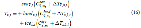
The temperature climatology of sea regions Csea, the temperature climatology of land regions Cland, and the temperature climatology of sea ice regions Cice were estimated as
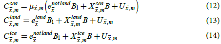
where  is a function that returns the HadSST3 climatology at for calendar month m if it is available, but is otherwise the identity
function,
is a function that returns the HadSST3 climatology at for calendar month m if it is available, but is otherwise the identity
function,  is the average land elevation at , and
  is
the average surface elevation of non-land regions at . Csea mostly
reflects the HadSST3 climatology, except for a few grid cells where the
HadSST3 climatology is not available.
is
the average surface elevation of non-land regions at . Csea mostly
reflects the HadSST3 climatology, except for a few grid cells where the
HadSST3 climatology is not available.
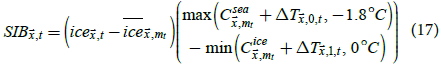
Sea ice bias can be estimated as the change in SIF multiplied by the difference between sea temperatures and sea ice temperatures. For this study, sea ice bias was estimated as
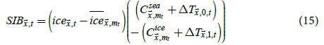
where  is the sea ice bias at for month t,
  is the SIF at for month t. Sea ice bias-corrected temperatures of grid cells were
estimated as
is the SIF at for month t. Sea ice bias-corrected temperatures of grid cells were
estimated as
Temperatures inferred using (15) may be physically unrealistic, such as inferred sea temperatures below the freezing temperature of sea water or inferred sea ice temperatures above the freezing temperature of fresh water. Therefore, one may want to use the following to estimate sea ice bias while preventing unphysical temperatures.
Bias-corrected temperatures that are physically realistic could then be estimated as
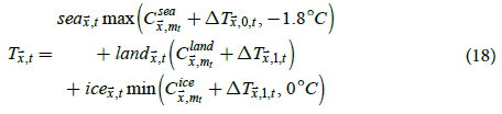
The maximum function restricts temperatures of sea water to at least -1.8°C, which is the freezing temperature of sea water with a salinity of 35 parts per thousand, and the minimum function restricts temperatures of sea ice at most 0°C. which is the freezing temperature of fresh water. While SATs above sea and sea ice can exceed these limits, they cannot significantly exceed these limits for monthly temperature averages. Restricting sea temperatures to at least -1.8°C is standard practice and is performed in HadISST1, KOBE-SST1 [35], ERSSTv5 [4], and BEST. Also, sea ice regions tend to have isothermal summers with temperatures close to 0°C [22].
While sea ice bias and temperature estimates using (17) and (18) would be physically realistic, they might be statistically biased. Estimating (9) and (11) using MLE would correspond to B being estimated using generalized least squares (GLS) given the estimate of the covariance function. GLS is unbiased if the covariance function is known; therefore, estimates of (15) and (16) may be relatively unbiased. Applying minimum and maximum functions to GLS estimates could result in biased estimates; in particular, the magnitude of sea ice bias could be overestimated. In addition, it is unclear if the use of freezing temperatures in (17) and (18) is appropriate as the temperature climatology datasets used have measurement error and do not correspond perfectly with the temperature anomaly datasets. Therefore, the results of (15) and (16) are presented as the main estimates of this study and the results of (17) and (18) are presented as alternate estimates.
Changes in SICs can cause changes in local temperatures. Changes in local temperatures can cause changes in SICs. In addition, changes in SICs can cause temperature changes in nearby regions due to heat transfer. The sea ice bias estimated using the above methodology may capture all three of these mechanisms and does not necessarily reflect the impact of SICs on local temperatures alone. This lack of distinction of these mechanisms in the statistical model can make physically interpretability of results difficult. However, for the purpose of statistically inferring temperatures using available data, it is not necessary to identify how much of the correlation between SICs and local temperatures is caused by each of these mechanisms since what matters is the existence of the correlation.
If SICs are correlated with the temperatures of nearby regions and if the statistical model used assumes a temperature field that is discontinuous between sea and sea ice regions, then this could cause an overcorrection for sea ice bias. This is because the temperature anomaly observations of nearby land or sea regions may already reflect the higher regional warming due to melting sea ice. If the temperature climatology function is estimated from blended data and a coarse resolution is used, then this may cause the temperature climatology model to overestimate the impact of SICs on local temperatures, resulting in a further overcorrection for sea ice bias. To test for this potential issue, IABP-POLES data north of 60°N was used. Using ordinary least squares, the temperature climatology function was re-estimated twice: once using a 5° resolution of IABP-POLES and once using a 1° resolution of IABP-POLES. For simplicity, these tests neglect differences in ΔT between land-ice and sea regions in (15). The impact of sea ice bias on the GMST due to changes in SICs north of 60°N was estimated for each of these resolutions. To be consistent with Jones et al, IABP-POLES were treated as a 1961-1990 climatology.
As an additional test, empirical LAFs of regions of sea ice loss were calculated for HadCRU_MLE and for CCSM4 under the RCP6.0 scenario using a 5° resolution. For each calendar month, weighted averages of temperature change from the late 1800s to 2018, weighted by the surface area of net sea ice loss for each grid cell, were calculated. These weighted temperature changes were averaged over the calendar year and divided by the annual GMST change to produce empirical LAFs of regions of sea ice loss. For simplicity, leap days were neglected in this calculation. While these empirical LAFs may underestimate the true LAF of regions of sea ice loss due to using a coarse resolution of 5°, they provide useful metrics for comparison.
For each of the temperature climatology models, its uncertainty was evaluated using a Monte Carlo approach. The Monte Carlo approach produced 200 ensemble members of temperature climatologies. To generate these ensemble members, each of the 100 ensemble members of the HadSST3 climatology was used twice. The HadSST3 ensemble accounts for bias uncertainties, but not other uncertainties such as measurement or sampling uncertainties. 200 ensemble members of sea ice bias and 200 ensemble members of blended temperatures were then calculated. While this Monte Carlo approach accounts for parameter estimation uncertainty and infilling uncertainty, bias and uncertainty due to a possible methodological overcorrection for sea ice bias were neglected. In addition, measurement uncertainties of temperature climatologies and uncertainties of SICs were neglected since they were not quantified. Uncertainties of SICs may be large as SICs vary greatly between datasets; the change in average global sea ice extent between the late 1800s and 2018 is -0.7% of the Earth’s surface according to HadISST1, which is approximately half of the -1.3% change according to HadISST2.
Patterns of Internal Variability
Temperature patterns that correspond to modes of internal variability are needed to use (7) to obtain amplification bias-corrected estimates of past temperatures. One approach to obtain IVPs is to use the method of empirical orthogonal teleconnections (EOTs) [36]. This is used extensively by NOAA in ERSSTv5, where 140 EOTs are used to reconstruct SSTs. NOAA calculates its EOTs using OISSTv2 [37] data for the period 1982-2011. OISSTv2 combines satellite data with SST data and is spatially complete. A second approach is to use empirical orthogonal functions (EOFs) [38]. Methodologies where one first obtains internal variability indices from observed temperatures and then looks for IVPs that are orthogonal to these indices have also been used [24,39,40].
The approach of NOAA of using OISSTv2 data to calculate IVPs has three problems. Firstly, as global warming has occurred over the instrumental period, estimates of these IVPs might contain warming signals. Secondly, estimates of these IVPs are not independent of instrumental temperature data, thus proper error analysis using these IVPs becomes more difficult. Thirdly, estimates of these IVPs include weather residuals for the period 1982-2011. Thus, the use of such estimated IVPs in (7) could result in zero-biased estimates of internal variability indices due to attenuation bias [41]. Even worse, because of how such IVPs are calculated, estimates of internal variability indices could contain more attenuation bias prior to 1982 than after 1982, which might affect estimates of changes in ENSO variability over time. The use of climate model output for scenarios with constant forcing over time can avoid these three problems. This approach has been performed using CMIP5 output for pre-industrial control scenarios [24,39,40].
Warmer temperatures due to internal variability can cause sea ice to melt, which could cause high localized warming in areas where sea ice melts. However, the correlation between SICs and temperature is included in the correction for sea ice bias. If IVPs include temperature changes explained by SIC changes, then this could result in double counting. Therefore, it is desirable to remove temperature changes explained by SIC changes from temperature anomalies before obtaining IVPs.
To remove temperature changes explained by SIC changes, the results of the best climatology model estimated using Jones et al. data were used. In particular, sea ice detrended temperature anomalies for CCSM4 under the pre-industrial control scenario were estimated as

where  is the CCSM4 temperature anomaly at for month t,
and
is the CCSM4 temperature anomaly at for month t,
and  is the detrended temperature anomaly at for month t.
SICs of CCSM4 were used for ice and
is the detrended temperature anomaly at for month t.
SICs of CCSM4 were used for ice and  whereas the ensemble of the
best temperature climatology model estimated using Jones et al. data
was used for Csea and Cice.
whereas the ensemble of the
best temperature climatology model estimated using Jones et al. data
was used for Csea and Cice.
EOFs were calculated from annual averages of the ensemble median of detrended CCSM4 temperature anomalies using the approach given in the supplementary information. Annual averages were used to remove temperature variation on a timescale of less than a year. Throughout this study, annual averages were calculated by weighted each month by its number of days while accounting for leap years. An EOF approach was used instead of an EOT approach since the EOT approach would involve the selection of a set of reference grid cells, which can be somewhat arbitrary.
Results and Discussion
Table 5 summarizes the results of the estimated temperature anomaly models. For the best (lowest AIC) model with a constant amplification function (amplification function 1), the maximum likelihood estimate of GMST change from the late 1800s to 2018 is 1.11°C, which is similar to the 1.11°C estimate of GMST change of C&W. When the best amplification function is introduced into the model, the estimate of GMST change increases by 0.01°C to 1.12°C. This is expected as polar regions, which tend to be poorly observed, have high LAFs. Introducing the IVP for ENSO leaves the estimate of GMST change relatively unchanged at 1.12°C. For the best temperature anomaly model, the maximum likelihood estimate of GMST change is slightly greater than the ensemble median estimate of GMST change: 1.11°C, with a 95% confidence interval of (1.04°C, 1.20°C).
Table 5: Summary of results of the estimated temperature anomaly models. Estimates listed correspond to maximum likelihood estimates. The global mean surface temperature (GMST) change values listed in this table do not correct for sea ice bias and include the impact of the internal variability pattern (IVP) if applicable.
| Amplification function | Covariance function | Number of IVPs |
nAIC | nBIC | GMST change from the late 1800s to 2018 (°C) | Correlation of residuals between consecutive months | Correlation decay length (km) | Correlation of residuals between land-ice and sea regions |
|---|---|---|---|---|---|---|---|---|
| 1 | 1 | 0 | 2.279 | 2.288 | 1.103 | 0.08 | 970 | 0.36 |
| 1 | 2 | 0 | 2.194 | 2.203 | 1.107 | 0.08 | 975 | 0.53 |
| 2 | 2 | 0 | 2.194 | 2.203 | 1.108 | 0.08 | 974 | 0.53 |
| 3 | 2 | 0 | 2.194 | 2.203 | 1.106 | 0.08 | 974 | 0.53 |
| 4 | 2 | 0 | 2.194 | 2.203 | 1.116 | 0.08 | 969 | 0.53 |
| 4 | 2 | 1 | 2.190 | 2.207 | 1.117 | 0.07 | 945 | 0.52 |
Figure 1 shows averages of the estimated amplification functions for each meteorological season; for simplicity, amplification functions are shown by meteorological season instead of by calendar month. As expected, polar regions tend to have higher estimated LAFs than equatorial regions and land-ice regions tend to have higher estimated LAFs than sea regions. The northern hemisphere tends to have higher estimated LAFs than the southern hemisphere.

Figure 1: Weighted average of the maximum likelihood estimates of local amplification factors by meteorological season: (a) December-January-February, (b) March-April-May, (c) June-July-August, and (d) September-October-November. Calendar months were weighted by their average number of days. These estimated local amplification factors neglect changes in sea ice. The shaded areas correspond to the 95% confidence regions.
The estimated LAFs are often far from unity, with arctic land regions having LAFs of two or greater. This suggests that accounting for LAFs is important for temperature estimates of unobserved regions. Of the GITDs discussed in the introduction, none of their statistical models adequately account for LAFs, so all should be subject to amplification bias. GISTEMPv4 and NOAAGlobalTempv5 use ERSSTv5 for SSTs; ERSSTv5 might indirectly account for some amplification bias through its use of EOTs. In addition, GISTEMPv4 averages temperature anomalies zonally before averaging globally, which may cause GISTEMPv4 to have reduced amplification bias compared to other GITDs.
Figure 2 shows the first EOF of the CCSM4 detrended temperature anomalies under the pre-industrial control scenario. This EOF appears to correspond to the temperature pattern of ENSO due to its strong warming band in the Eastern Equatorial Pacific. If temperature variation explained by SICs is excluded, this EOF explains 18% of the variation in local annual mean SATs and 51% of the variation in annual GMSTs for the CCSM4 output under the pre-industrial control scenario.

Figure 2: The dominant temperature pattern of internal variability obtained from CCSM4 output under the pre-industrial control scenario. The strong warming band in the Eastern Equatorial Pacific suggests that this pattern corresponds to the El Niño Southern Oscillation.
Figure 3 shows the estimated impact of the IVP on annual GMST anomalies. It appears that this IVP causes fluctuations in annual GMSTs with an amplitude of approximately 0.1°C. The GMST variability explained by this IVP corresponds well with the SOI, suggesting that this mode of internal variability corresponds well to ENSO.

Figure 3: Maximum likelihood estimate of the impact of the internal variability pattern on annual global mean surface temperature (GMST) anomalies using 1961-1990 as the reference period. This estimate neglects the indirect impact on the GMST due to how internal variability may affect sea ice concentrations. The internal variability pattern corresponds well with the negative of the Southern Oscillation Index, suggesting that this mode of internal variability corresponds to the El Niño Southern Oscillation. The gray area corresponds to the 95% confidence region.
Table 6 summarizes the results of the estimated temperature climatology models. For the model with the lowest AIC, the median estimate of the impact of sea ice bias on GMST change from the late 1800s to 2018 is -0.08°C, with a 95% confidence interval of (-0.04°C, -0.13°C). The maximum likelihood estimate of the lapse rate of the best model is 6.4°C km-1, corresponding to a typical wet lapse rate for Earth; the retrieval of a physically sensible lapse rate adds confidence to the results of the temperature climatology model. When the freezing temperatures of sea water and fresh water are applied, the median estimate of GMST change remains relatively unchanged at -0.09°C. Thus, while the use of the freezing temperatures has an impact on the estimated bias, it does not change the order of magnitude of estimated bias.
Table 6: Summary of results of the estimated temperature climatology models. The best (lowest nAIC) temperature anomaly model of Table 5 was used in the estimation of the impact of sea ice bias on global mean surface temperature (GMST) change. Sea ice bias estimates listed correspond to ensemble median estimates; other estimates listed correspond to maximum likelihood estimates.
Climatology function |
Covariance function | nAIC | nBIC | Impact of sea ice bias on the GMST change from the late 1800s to 2018 (°C) |
Correlation of residuals between calendar months | Correlation decay length (km) | Lapse Rate (°C km-1) | |
|---|---|---|---|---|---|---|---|---|
| Neglecting freezing temperatures |
Using freezing temperatures | |||||||
| 1 | 1 | 2.21 | 2.22 | -0.067 | -0.070 | 0.67 | 2481 | 5.86 |
| 1 | 2 | 1.74 | 1.76 | -0.063 | -0.063 | 0.70 | 2879 | 6.10 |
| 1 | 3 | 2.03 | 2.04 | -0.064 | -0.070 | 0.78 | 2506 | 6.36 |
| 1 | 4 | 1.56 | 1.58 | -0.063 | -0.063 | 0.75 | 2906 | 6.47 |
| 2 | 4 | 1.54 | 1.56 | -0.094 | -0.097 | 0.74 | 2334 | 6.46 |
| 3 | 4 | 1.50 | 1.54 | -0.086 | -0.089 | 0.74 | 2315 | 6.41 |
| 4 | 4 | 1.55 | 1.57 | -0.063 | -0.064 | 0.74 | 2924 | 6.44 |
| 5 | 4 | 1.51 | 1.54 | -0.092 | -0.094 | 0.75 | 2210 | 6.45 |
| 6 | 4 | 1.47 | 1.53 | -0.091 | -0.094 | 0.75 | 2228 | 6.40 |
To test for a possible overestimation of sea ice bias due to using a temperature field that is discontinuous between sea and sea ice regions, the climatology function was re-estimated twice using IABP-POLES. When the resolution is 5° and when only accounting for changes in sea ice north of 60°N, the estimate of the impact of sea ice bias on GMST change between the late 1800s and 2018 is -0.045°C. When the resolution is changed to 1°, the estimate is reduced in magnitude to -0.030°C. Since the use of a coarser resolution should result in a greater overestimation of sea ice bias, this suggests that there could be could result in a 50% overestimation of sea ice bias. In addition, some overestimation may remain as a 1° resolution is still somewhat coarse.
As an additional test, empirical LAFs of regions of sea ice loss from the late 1800s to 2018 were calculated. Combining the best temperature anomaly model with the best temperature climatology model constructs HadCRU_MLE. According to HadCRU_MLE, the median estimate of the empirical LAF is 1.5 if no sea ice bias correction is included and 4.6 if the sea ice bias correction is included. In comparison, the empirical LAF is 2.7 for CCSM4 under the RCP6.0 scenario using a 5° resolution. This suggests that while a sea ice bias correction is needed, HadCRU_MLE may overcorrect for sea ice bias by a factor of two.
Both local observations of temperatures in sea ice regions as well as results of climate models can help quantify the magnitude of sea ice bias. Rayner et al. [19] use local temperature observations to estimate the relationship between temperature and SIC. Figure 7, I estimate by visual inspection that the difference in temperature in going from 0% SIC to 100% SIC is likely between 2°C and 6°C. Multiplying this by the change in average global sea ice extent between the late 1800s and 2018 suggests a sea ice bias of between -0.03°C and -0.08°C. Alternatively, Cowtan et al. [32] find, using CMIP5 output, that blending land and sea absolute temperatures instead of blending land and sea temperature anomalies increases the estimated GMST change by 3%. Since the GMST change over the instrumental period is approximately 1°C, this suggests that sea ice bias may cause an underestimation of GMST change of 0.03°C. Thus, both local observations of temperatures in sea ice regions and results of climate models confirm the order of magnitude of sea ice bias estimated in this study.
Figure 4 shows the estimated impact of sea ice bias on annual GMST anomalies. Figure 5 shows the distribution of the estimated impact of sea ice bias on surface temperature change from the late 1800s to 2018. Regions that have experienced significant ice melt over the instrumental period, such as the Norwegian Sea and parts of the Southern Ocean, show the most bias.

Figure 4: Ensemble median estimates of the impact of sea ice bias on estimates of annual global mean surface temperature (GMST) anomalies using 1961- 1990 as the reference period. The gray area corresponds to the 95% confidence region.

Figure 5: Ensemble median estimates of the impact of sea ice bias on the change in local surface temperature (°C) from the late 1800s to 2018.
It should be noted that HadISST2 is imperfect. In the northern hemisphere, it has no interannual change in SICs prior to 1901 and little interannual change in SICs prior to 1953. In the southern hemisphere, it has no interannual change in SICs prior to 1939 and little interannual change in SICs prior to 1973. This is caused by a lack of data and infilling missing data with SIC climatologies estimated using data from other years. As a result, HadISST2 underestimates SIC change prior to 1973. Thus, the results of this study likely underestimate variation in sea ice bias prior to 1973.
The results of HadCRU_MLE give this study’s best estimate of GMST change from the late 1800s to 2018: 1.20 ° C with a 95% confidence interval of (1.11 ° C, 1.30 ° C). As an alternate estimate, if the freezing temperatures of sea water and fresh water are applied, then the median estimate of GMST change remains relatively unchanged at 1.20 ° C.
Figure 6 shows this study’s best estimates of annual GMST anomalies. Figure 7 shows the distribution of local surface temperature change from the late 1800s to 2018. HadCRU_MLE estimates more warming than the 1.16°C of GMST change from the late 1800s to 2018 of BEST. This may be because BEST uses HadSST3, which shows less warming over the instrumental period than HadSST4. The estimate of GMST change increases from 1.03°C in C&W-HadSST3 to 1.11°C in C&W, suggesting that the estimate of GMST change of BEST would increase by a comparable amount if it is updated to use HadSST4. As BEST accounts for changes in SICs, the larger estimate of GMST change of BEST compared to C&W is partially explained by the sea ice bias of C&W; the remaining difference could be due to different homogenization procedures of LSATs or differences in statistical infilling methods.

Figure 6: Ensemble median estimates of annual global mean surface temperature anomalies using 1961-1990 as the reference period. The figure shows the best estimates of this study (HadCRU_MLE) compared to the results of Cowtan and Way version 2 using HadSST4. The gray area corresponds to the 95% confidence region.

Figure 7: Ensemble median estimates of the change in local surface temperature (°C) from the late 1800s to 2018.
Figure 7 shows a large contrast in temperature change in the Southern Ocean. This contrast is likely exaggerated since HadISST2 neglects interannual variation in SICs for the late 1800s. The large change in SICs for the Southern Ocean is largely the result of a single German 1929-1939 Antarctic sea ice climatology. Thus, the reliability of this study’s estimate of temperature change since the late 1800s for the Southern Ocean is largely dependent on this single 1929-1939 temperature climatology.
HadCRU_MLE may have a remaining bias due to using SSTs instead of MATs. According to the results of climate models, this bias may cause an underestimation of GMST change of 5% to 9% [32,33]. However, the top ocean layer of climate models is typically 10 m deep, whereas the SSTs of HadSST4 use a buoy reference depth 20 cm below the sea surface; so, the actual bias of HadCRU_MLE should be smaller than the bias suggested by climate models. In addition, HadSST4 assumes that MATs and SSTs warm at similar rates and uses MATs to correct for SST biases. In particular, MATs are used to determine the fractions of canvas and wooden buckets in the early part of the instrumental period. So, it is unclear if there is any significant bias due to differences in warming rates of SSTs and MATs when using HadSST4.
While this paper outlines some improvements to the statistical methodology of estimating past temperatures, there are still areas where further improvements could be made. Firstly, uncertainties in the estimates of the temperature climatology and SICs could be quantified and taken into account. Secondly, the magnitude of sea ice bias could be better quantified and verified using different lines of evidence. Thirdly, attempts to better incorporate bias errors of instrumental observations into the statistical model could be made. Fourthly, amplification and temperature climatology functions of this study are discontinuous between land-ice and sea regions, which are physically unrealistic; further improvements to the functional forms could be made. Lastly, other sources of observations, such as satellite and paleoclimate data, could be used to further improve temperature estimates.
Conclusions
This paper identifies two biases in GITDs: amplification bias and sea ice bias. Amplification bias occurs when the underlying statistical model of the GITD neglects the tendency of different regions of the planet to warm at different rates. Since polar regions, which tend to warm the fastest, were poorly observed during the instrumental period, not accounting for amplification bias causes an underestimation of GMST change over the instrumental period. Sea ice bias occurs when the GITD neglects the impact of changes in sea ice on temperatures. Since SICs have decreased over the instrumental period, neglecting changes in SICs causes an underestimation of GMST change over the instrumental period. To quantify the impact of these biases, a new bias-corrected GITD was constructed, called HadCRU_MLE, which used MLE to combine the LSAT anomalies of HadCRUT4 with the SST anomalies of HadSST4.
HadCRU_MLE has improvements compared to C&W. Model parameters were estimated using MLE, which provides a better statistical foundation for parameter estimates and allows for quantification of parameter uncertainty. HadCRU_MLE takes advantage of temporal correlations and correlations between landice and sea regions to improve temperature anomaly estimates. More sources of uncertainty are accounted for, including parameter estimation uncertainty and infilling uncertainty as well as all uncertainties of HadCRUT4 and HadSST4.
To correct for amplification bias, an amplification function was incorporated into the temperature anomaly model, which was fit to observations. As El Niño events correspond to warming concentrated in the Eastern Equatorial Pacific Ocean, neglecting the behaviour of ENSO could cause an attenuation bias towards the identity function of the estimate of the amplification function. To avoid this attenuation bias, an IVP for ENSO was obtained from CCSM4 output for a preindustrial control scenario and incorporated into the temperature anomaly model. The inclusion of the amplification function and the IVP for ENSO increases the estimate of GMST change from the late 1800s to 2018 by 0.01°C.
To correct for sea ice bias, a temperature climatology model was fit to observations. Estimates of temperature climatologies and temperature anomalies were combined to quantify sea ice bias. Accounting for sea ice bias increases the estimate of GMST change from the late 1800s to 2018 by 0.08°C. The use of a temperature field that is discontinuous between sea and sea ice regions may cause an overcorrection for sea ice bias. The results of sensitivity tests using IABP-POLES data suggest that there may be a 50% overcorrection for sea ice bias. A comparison of HadCRU_MLE with CCSM4 output under the RCP6.0 scenario, which roughly corresponds to historic forcing, suggests that there may be an overcorrection by a factor of two for sea ice bias. Overall, the median estimate of GMST change from the late 1800s to 2018 is 1.20°C, with a 95% confidence interval of (1.11°C, 1.30°C).
Acknowledgments
I thank all who contributed to the source datasets used in this study, the editor and reviewers of this paper, the World Data Center for Climate at DKRZ for archiving the code and data of HadCRU_MLE [42], and Steven Mosher and Kevin Cowtan for providing inspiration. This research received no funding.
References
- Morice P, Kennedy J, Rayner A, Jones D (2012) Quantifying Uncertainties in Global and Regional Temperature Change using an Ensemble of Observational Estimates: The HadCRUT4 Dataset. J Geophys Res Atmos. 117: 101
- Lenssen L, Schmidt A, Hansen E, Menne J, Persin A, et.al. (2019) Improvements in the GISTEMP uncertainty model. J Geophys Res Atmos. 124: 6307-6326
- Vose S, Arndt D, Banzon F, Easterling R, Gleason E, et al. (2012) NOAA’s Merged Land-Ocean Surface Temperature Analysis. Bull Am Meteorol Soc. 93: 1677-1685
- Huang B, Thorne W, Banzon F, Boyer T, Chepurin G, et al. (2017) Extended Reconstructed Sea Surface Temperature version 5 (ERSSTv5), Upgrades, validations, and intercomparisons. J Clim. 30: 8179-8205
- Menne J, Williams N, Gleason E, Rennie J, Lawrimore H, et.al. (2018) The Global Historical Climatology Network Monthly Temperature Dataset, Version 4. J Clim. 31: 9835-9854
- Krige G (1951) A Statistical Approach to some Basic Mine Valuation Problems on the Witwatersrand. J Chem Metall Min Soc S Afr. 52: 119-139
- Matheron G (1962) Traité de Géostatistique Appliquée (Vol 1). Éditions Technip, Paris, France
- Rohde R, Muller A, Jacobsen R, Muller E, Perlmutter S, et al. (2013) A New Estimate of the Average Earth Surface Land Temperature Spanning 1973 to 2011. Geoinf Geostat Overview 1
- Rohde R, Muller A, Jacobsen R, Perlmutter S, Rosenfeld A, et al. (2013) Berkeley Earth Temperature Averaging Process. Geoinf Geostat Overview 1
- Rohde RA, Hausfather Z (2020) The Berkeley Earth Land/Ocean Temperature Record. Earth Syst Sci Data 12: 3469-3479
- Cowtan K, Way G (2014) Coverage Bias in the HadCRUT4 Temperature Series and its Impact on Recent Temperature Trends. Q J R Meteorol Soc. 140: 1935-1944
- Cowtan K, Way G (2014) Coverage Bias in the HadCRUT4 Temperature Series and its Impact on Recent Temperature Trends. UPDATE. Temperature Reconstruction by Domain: Version 2.0 Temperature Series. University of York Press, York, UK
- Kennedy J, Rayner A, Smith O, Parker E, Saunby M, et.al. (2011) Reassessing Biases and Other Uncertainties in Sea-Surface Temperature Observations since 1850 Part 1: Measurement and Sampling Errors. J Geophys Res Atmos. 116: 14103.
- Kennedy J, Rayner A, Smith O, Parker E, Saunby M, et.al. (2011) Reassessing Biases and Other Uncertainties in Sea-Surface Temperature Observations since 1850 Part 2: Biases and Homogenisation. J Geophys Res Atmos. 116: 14104
- Kennedy J, Rayner A, Atkinson P, Killick E (2019) An ensemble data set of sea surface temperature change from 1850: the Met Office Hadley Centre HadSST.4.0.0.0 data set. J Geophys Res Atmos. 124: 7719-7763
- Akaike H (1974) A New Look at the Statistical Model Identification. IEEE Trans Automat Contr. 19: 716-723
- Jones D, Lister H, Osborn J, Harpham C, Salmon M, et al. (2012) Hemispheric and Large-scale Land Surface Air Temperature Variations: An Extensive Revision and an Update to 2010. J Geophys Res Atmos 117: D05127
- Donlon J, Marin M, Stark J, Roberts-Jones J, Fiedler E, et al. (2011) The Operational Sea Surface Temperature and Sea Ice Analysis (OSTIA). Remote Sens Environ. 116: 140-158
- Rayner A, Parker E, Horton B, Folland K, Alexander V, et al. (2003) Global Analyses of Sea Surface Temperature, Sea Ice, and Night Marine Air Temperature since the Late Nineteenth Century. J Geophys Res Atmos. 108: 4407.
- Titchner A, Rayner A (2014) The Met Office Hadley Center Sea Ice and Sea Surface Temperature Data Set, Version 2: 1. Sea Ice Concentrations. J Geophys Res Atmos. 119: 2864-2889.
- Jones D, New M, Parker E, Martin S, Rigor G, et.al. (1999) Surface Air Temperature and its Changes over the Past 150 Years. Rev Geophys. 37: 173-199
- Rigor G, Colony L, Martin S (2000) Variations in surface air temperature in the Arctic from 1979-1997. J Clim 13: 896-914
- Danielson J, Gesch B (2011) Global multi-resolution terrain elevation data 2010 (GMTED2010). US Geol Surv Open-File Rep: 2011-1073
- Meehl A, Hu A, Santer D, Xie P (2016) Contribution of the Interdecadal Pacific Oscillation to Twentieth-Century Global Surface Temperature Trends. Nat Clim Change 6: 1005-1008.
- Ropelewski F, Jones D (1987) An Extension of the Tahiti-Darwin Southern Oscillation Index. Mon Weather Rev 115: 2161-2165.
- Serreze C, Barry G (2011) Processes and impacts of arctic amplification: A research synthesis. Glob Planet Change 77: 85-96.
- Cohen J, Screen A, Furtado C, Barlow M, Whittleston D, et al. (2014) Recent arctic amplification and extreme mid-latitude weather. Nat Geosci 7: 627-637.
- Stjern W, Lund T, Samset H, Myhre G, Forster M, et al. (2019) Arctic Amplification Response to Individual Climate Drivers. J Geophys Res Atmos 124: 6698-6717.
- Pascanu R, Dauphin YN, Ganguli S, Bengio Y (2014) On the Saddle Point Problem for Non-Convex Optimization.
- Dauphin N, Pascanu R, Gulcehre C, Cho K, Ganguli S, et al. (2014) Identifying and Attacking the Saddle Point Problem in High-Dimensional Non-Convex Optimization. Proceedings of Advances in Neural Information Processing Systems 27 (NIPS 2014).
- Schwarz G (1978) Estimating the Dimension of a Model. Ann Stat 6: 461-464.
- Cowtan K, Hausfather Z, Hawkins E, Jacobs P, Mann ME, et al. (2015) Robust Comparison of Climate Models with Observations using Blended Land Air and Ocean Sea Surface Temperatures. Geophys Res Lett 42: 6526-6534.
- Richardson M, Cowtan K, Hawkins E, Stolpe MB (2016) Reconciled Climate Response Estimates from Climate Models and the Energy Budget of Earth. Nat Clim Change 6: 931-935.
- New M, Hulme M, Jones P (1999) Representing Twentieth-Century Space-Time Climate Variability. Part I: Development of a 1961-90 Mean Monthly Terrestrial Climatology. J Clim 13: 2217-2238.
- Ishii M, Shouji A, Sugimoto S, Matsumoto T (2005) Objective Analyses of Sea-Surface Temperature and Marine Meteorological Variables for the 20th Century using ICOADS and the Kobe Collection. Int J Climatol 25: 865-879.
- van den Dool M, Sasha S, Johansson Å (2000) Empirical Orthogonal Teleconnections. J Clim 13: 1421-1435
- Reynolds W, Rayner A, Smith M, Stokes C, Wang W (2002) An Improved In Situ and Satellite SST Analysis for Climate. J Clim 15: 1609-1625.
- Lorenz N (2015) Empirical Orthogonal Functions and Statistical Weather Prediction. Massachusetts Institute of Technology, Department of Meteorology, Cambridge, USA
- Huber M, Knutti R (2014) Natural variability, radiative forcing and climate response in the recent hiatus reconciled. Nat Geosci 7: 651-656.
- Stolpe B, Medhaug I, Knutti R (2017) Contribution of atlantic and pacific multidecadal variability to twentieth-century temperature changes. J Clim 30: 6279-6295.
- Riggs S, Guarnieri A, Addelman S (1978) Fitting straight lines when both variables are subject to error. Life Sci 22: 1305-1360.
- Calvert T (2020) HadCRU_MLE_v1. World Data Center for Climate (WDCC) at DKRZ, Hamburg, Germany.