Spanish
  Chinese
  Russian
  German
  French
  Japanese
  Portuguese
  Hindi
Hindi Research Article, Geoinfor Geostat An Overview Vol: 7 Issue: 1
Evaluating Interpolation Methods by Geostatistical Modeling of the Douala Oil Field Porosity Data (Cameroon)
Jean Jacques Nguimbous-Kouoh1* and Eliezer Manguelle-Dicoum2
1Department of Mines, Petroleum, Gas and Water Resources Exploration, Faculty of Mines and Petroleum Industries, University of Maroua, Cameroon
2Department of Physics, Faculty of Science, University of Yaoundé I, Cameroon
*Corresponding Author : Jean Jacques Nguimbous-Kouoh
Department of Mines, Petroleum, Gas and Water Resources Exploration, Faculty of Mines and Petroleum Industries, University of Maroua, Cameroon
Tel: (+237) 696 383 408
E-mail: nguimbouskouoh@yahoo.fr
Received: February 02, 2019 Accepted: February 19, 2019 Published: February 28, 2019
Citation: Nguimbous-Kouoh JJ, Manguelle-Dicoum E (2019) Evaluating Interpolation Methods by Geostatistical Modeling of the Douala Oil Field Porosity Data (Cameroon). Geoinfor Geostat: An Overview 7:1. doi: 10.4172/2327-4581.1000203
Abstract
The choice of an interpolation method to re-sample and solve the problem of scattered data is often difficult, as several methods show large differences in results. In this study, we re-sampled the sparsely porous data using three interpolation techniques: the inverse distance to a power, minimum curvature and kriging. The experimental variogram of field data was generated. The anisotropy of these data has been simulated by the Gaussian model and we have concluded that these data present a geometric anisotropy. The interpolated variograms from the three techniques were plotted and fitted by the least squares method. These variograms gave a better accuracy and consistency than the field data variogram. The accuracy and performance of the interpolation techniques were evaluated by calculating their Variance, their Skewness, their Kurtosis and their Root-mean-squared. Contour maps and Wireframes were also computed from interpolated grids to perform a visual analysis of the porosity spatial distribution. Porosity distribution of the studied field has a higher continuity in NE-SW direction.
Keywords: Porosity; Geostatistics; Modeling; Variograms; Douala Basin
Introduction
Geostatistics is a branch of statistics centered on spatial or spatiotemporal datasets. Originally developed to predict probability distributions of ores during mining operations [1-3], it is currently applied in various disciplines: petroleum geology, hydrogeology, hydrology, geochemistry, environmental control, landscape ecology [4-11]. The main originality of the geostatistical approach is that it uses spatialized data. These main aspects are [12-16]: considering the spatial structure of the data, the space of any dimension, the irregular and incomplete sampling of the fragmentary data and the considering of external information. Geostatistics is intimately related to interpolation methods, but extends far beyond simple interpolation problems. Geostatistical techniques are based on statistical models based on the theory of random variables. They help to know the uncertainty associated with spatial estimation [15,17]. A number of simpler interpolation methods/algorithms, such as inverse distance, minimum curvature, bilinear interpolation, and nearestneighbor interpolation, were already well known before geostatistics [1,2,4,8]. The choice of an interpolation method is difficult because some methods show large differences in results. The divergences between the results of the interpolation are mainly consequences of the following circumstances [12-16]: The available data sources are approximate for distribution, density and accuracy; The selected interpolation algorithm is not robust enough for the data used; The chosen interpolation algorithms or the data structure are not adapted to the field; The perception or interpretation of the operator; The properties of the sampling network and the spatial dependence of the variable of interest.
The aim of this study is to re-sample the scattered porosity data of a part of the Douala sedimentary basin by using three interpolation methods and investigate their patterns of spatial variability.
We present in this study, the study area data collection in the Douala sedimentary basin, the different interpolations methods and their mathematical formulation in the univariate framework. A variographic analysis of the field data will be performed. The simulations will be made from the field data variogram; the field data anisotropy will be tested. This analysis will spatially characterize the distribution of porosity at the measurement site. The grids of the data resampled by the interpolation techniques will be created. Then the interpolated variograms will be analyzed and their modeling quality will be evaluated and compared.
Location of the Study Area
Several authors have studied the application of geostatistics to the study of porosity in geological formations [15,17-22]. The porosity data used for this study come from the Douala sedimentary basin (Figure 1) which is a producing basin in Cameroon. The Douala Basin covers a total area of about 19000 km2 of which 7000 are emerged. The basin extends under the waters of the Gulf of Guinea by a continental platform with a width of 25 km. It includes two sub-basins [23]: the Douala sub-basin bounded on the north by the Cameroon volcanic line and on the south by the Nyong river and the Kribi-Campo sub-basin located north of the Ntem river. The region is marked by a relatively flat relief of an altitude not exceeding 200 m. The study area is located between latitudes 03°42’57’’N and 03°47’17’’N and longitudes 09°46’52’’ E and 09°52’16’’E.

Figure 1: Location map of the Douala Basin and the study area.
Data Source and Methods
Source of porosity data
Porosity data are often obtained by direct or indirect measurements. Laboratory measurements of porosity on cores are examples of direct methods. Porosity data from logs are considered indirect methods [17-20]. We use the porosity data collected from drilling logs (electrical, sonic, gamma radiation, porosity, density, photoelectric effect). They come from borehole wells whose depth varies between 355 m to 3024 m depth [24].
To re-sample the data, we used R and Surfer software’s [25]. Surfer is a 2D and 3D surface mapping program that transforms random data into contours of continuous curved faces. Surfer uses twelve different methods to interpolate data. However, in this case, only three methods were used.
The map (Figure 2) represents the classed post plot spatial porosity distribution above the study area. The porosity varies between 12% and 17%.

Figure 2: Classed post plot map of sample porosity data.
Methods
In linear geostatistics the choice of an interpolation method is very important to prove the spatial dependence of a variable of interest [1-4]. In this part, we present the interpolation methods from the uni-varied framework.
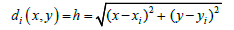
The Inverse distance to a power method: It is a deterministic method that consists in measuring the distance between the sought point and the known points around [25-29]. The calculation of the desired point is done by averaging the values of the surrounding points. Thus, the closer the point to be interpolated to a point whose value is known, the closer the value of the point to be interpolated is to the known value. The distance h between the sought point and the known points around is defined in the following way [26,28,30,31]:
And the result of the interpolation is:
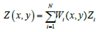
where Zi denotes the values taken by the point to be interpolated and Wi the associated weights:
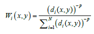
The weighting corresponds to the inverse of the distance 1/di with i > 0. The weights Wi are inversely proportional to a power p > 0 so that the data close to the studied point intervene more in the average than the more distant data. The factors that affect this method are the value of the power parameter p; the size of the study area and the number of neighbors. These factors are relevant to the accuracy of the results.
The minimum curvature method: The minimum curvature method has first been proposed by Briggs [32] for automatic contouring of geophysical data. It solves the problem to interpolate the data onto a regular grid in the sense that a grid point value tends to an observational value if the position of the observation tends to the grid point. For this a two-dimensional cubic spline is fit to the data by solving the corresponding difference equations, which have been set up under the conditions. The curvature is constructed directly in terms of the grid point values:
and depends on the grid spacing h. The discrete total squared curvature is
where: 
To minimize c, the partial derivatives of c with respect to F(xl,yk) must be set to zero. The resulting equations determine a set of relations between neighboring grid point values, one for each point. If one of the samples does not coincide with a grid point, additional difference equations are used for the grid points at the vertices of the square containing the sample, and the sampling point becomes part of the grid.
The resulting system of equations is then solved iteratively. The method is fast but has the disadvantage of being interpolating rather than approximating.
Kriging and variographic formalism: In a classical framework, kriging analysis generally involves two stages: the variogram estimation and the use of the coefficients of its model for kriging [33-37].
The formalism of variographic estimation: The variogram is a basic tool in kriging analysis and is required for geostatistical spatial prediction. The variogram is estimated by the experimental variogram γ*(h), which is calculated from the discrete data as follows [28]:
where N is the number of pairs of points distant from h.
Once the experimental variogram has been calculated, it is necessary to replace it with a theoretical variogram whose coefficients are estimated by a least squares procedure [31].
There are several types of theoretical variogram models used for kriging [30]:
The spherical variogram is characterized by:
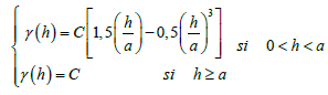
With a the range, h the lag of interpolation, C the constant sill
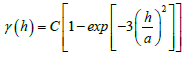
The Gaussian variogram is characterized by :
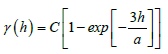
The exponential variogram is characterized by :
The variogram power is characterized by:
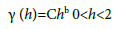
For b=1, the variogram is linear ; b=2. The variogram a is parabola
The formalism of variographic anisotropy: There are different types of anisotropies that can contaminate spatialized data [28]. Geometric anisotropy is the simplest case. A geometric anisotropy is reflected in the experimental variograms by a range which varies according to the direction. Geometric anisotropy is observed when the variogram respects the following mathematical formulation:
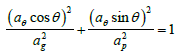
With ag the maximum range, ap the minimum range and aθ the range in the direction θ of the anisotropy.
Anisotropy is called zonal when it cannot be solved by a simple geometric or linear transformation of coordinates. It causes for the variogram a bearing which varies according to the direction of the space.
The kriging formalism
Kriging is an interpolation method that gives the best unbiased linear estimate of the point value of a regionalised variable [1-3]. The advantage of kriging is that it enables to calculate the estimation error, i.e. the variance of kriging [1-3]. It allows the considering of: the configuration of the data; the distance between data and targets; spatial correlations and external information. Kriging is an exact interpolator, it has a screen effect, and it is almost without conditional bias. It is transitive, generally performs a smoothing and considers the size of the field to be estimated and the position of the points between them [1-3].
The mathematical formulation of kriging imposes the minimization of the following variance [33,34,36]:

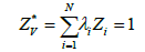
Where Zv represents the known values at certain points and:
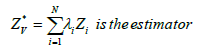
λi is the weight and Zi is the random variable corresponding to each point. Since kriging is an unbiased interpolator then:
To minimize the variance of kriging we use the Lagrangian [35]:
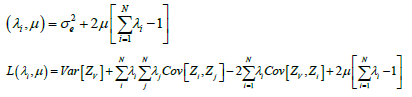
With μ the Lagrange multiplier.
By calculating: 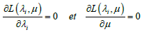 we obtain the system of equation:
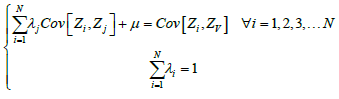
Solving this system of equation amounts to solving the following matrix system:
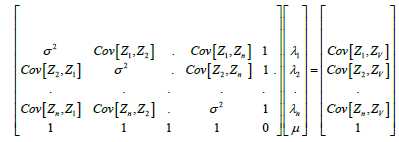
The system enables to find all the weights λ0 that minimize the variance and make the estimator unbiased. The variance of kriging is then obtained by the following formula:

The system of equations can also be expressed in terms of variogram under the assumption that the random process is stationary.
Results and Interpretation
In this part, we presented the different interpolated data grids, the variographic analysis and the porosity maps and wireframes obtained by the different methods.
Giddings interpretation
Figure 3(a-c) are the grids used to re-sample the data above the study area. The grids were made to have networks within which the interpolating routines can be applied. Gridding generally produces a regularly spaced array of Z values (porosity) from the irregularly spaced XYZ data.

Figure 3a: A view of grid nodes for porosity data of the inverse distance to a power.

Figure 3b: A view of grid nodes for porosity data of the minimum curvature.

Figure 3c: A view of grid nodes for porosity data of the kriging.
Figure 3a is the grid obtained by the inverse distance to a power method. This method is very sensitive to the number of used data and the value of the exponent, and a significant improvement in the accuracy of the estimate was obtained by selecting an optimal number of nearest neighbors and an optimal value of the exponent. This map was obtained by playing on the parameter p. This parameter determines how fast the weights fall with the distance from the grid node. The parameter p is a smoothing parameter. It allowed us to incorporate the uncertainty factor associated with our input data. The greater the smoothing parameter, the less the influence of a particular observation predominates in the prediction of a neighboring network node.
Figure 3b results from the grid made by the minimum curvature. The method is more precise when we specify the tensions and the number of iterations. Boundary and internal tensions were fitted to 0 to solve the biharmonic differential equation and produce the grid. They have been reduced to reduce overrun problems in sparse and unconstrained areas. The control of the convergence criteria has been carried out. When generating the grid, the maximum iteration value was kept at 100000 and the max residual at 0.0051.
Figure 3c results from the grid obtained by kriging. Kriging uses the variogram and assigns more influence to the nearest points in the interpolation of values for unknown locations. Kriging is an interpolation technique in which the surrounding measured values are weighted to derive a predicted value for an unmeasured location. Weights are based on the distance between the measured points, the prediction locations, and the overall spatial arrangement among the measured points. Kriging is unique among the interpolation methods in that it provides an easy method for characterizing the variance, or the precision, of predictions. Kriging is based on regionalized variable theory, which assumes that the spatial variation in the data being modeled is homogeneous across the surface. That is, the same pattern of variation can be observed at all locations on the surface. The variogram which enable to obtain this figure is of linear type with anisotropy of 1.
Variographic data analysis
Variogram analysis consists of the experimental variogram calculated from the data and the variogram model fitted to the data. The experimental variogram is calculated by averaging one-half the difference squared of the z-values over all pairs of observations with the specified separation distance and direction. It is plotted as a two-dimensional graph. Refer to formalism of variographic estimation for details about the mathematical formulas used to calculate the experimental variogram. The variogram model is chosen from a set of mathematical functions that describe spatial relationships. The appropriate model is chosen by matching the shape of the curve of the experimental variogram to the shape of the curve of the mathematical function [33-36].
Variogram analysis of field data: Figure 4 shows the scatter plot of the experimental variogram and the four types of theoretical models selected for its adjustment. Overall, all models lift first and then stabilize over greater distances beyond a certain range. The experimental variogram is a graph that shows the contributions of each pair of points to the final variogram. The scatter plot gives a visual impression of the dispersion of values at different offsets. He has no precise direction. The colored variograms were tested to find the variogram able of fitting the variographic cloud. This simulation shows that the yellow Gaussian variogram is the one that can best fit the field data. The directions and tolerances (Table 1) indicate the size of the angular window each time. We chose these directions and tolerances to obtain omnidirectional variograms that neglect the lag h.

Figure 4: Variographic cloud fitted by theoretical variograms.
| Model | Color | Sill | Range | Anisotropy ratio | Anisotropy angle | Slope | Variance | Tolerance | Direction | Power |
|---|---|---|---|---|---|---|---|---|---|---|
| Spherical | Blue | 1.155 | 18 | 1 | 0 | 0.142 | 1.155 | 45 | 45 | 0 |
| Gaussian | Yellow | 1.155 | 7 | 1.19exp-07 | 30 | 0.242 | 1.155 | 45 | 45 | 0 |
| Exponential | Red | 1.155 | 8.888 | 1 | 0 | 0.45 | 1.155 | 45 | 45 | 0 |
| Power | Green | No | 8 | 2 | 185 | 0.241 | 1.155 | 45 | 45 | 0.1 |
Table 1: Characteristics of the different variograms.
Table 1 shows the characteristics of the different theoretical variograms tested.
Field data anisotropy analysis: In the case of this simulation, the Gaussian model has been retained. Anisotropy is the parameter that allows us to better understand the correlation and spatial continuity of porosity values. Figure 5 shows the simulation of the theoretical variogram across the experimental variogram. This figure proves that field data has a geometric anisotropy. The three colored variograms have the same sill in all directions, identical nugget effect components, but different ranges from one direction to another. The maximum (ag) and minimum (ap) ranges are observed in two orthogonal directions. Spatial continuity is not necessarily the same in all directions. The three theoretical curves of this variogram form ellipsoids and fit the field data quite well because these data are only a sample of the actual porosity we wish to model. The interpolation will help us to perfectly model the porosity above the site.

Figure 5: Simulation of geometric anisotropy of field data.
Table 2 shows the characteristics of the different theoretical Gaussian models used to test geometric anisotropy of field data.
| Models | Color | Lag Weight | Tolerance | Direction | Anisotropy ratio | Anisotropy angle | Sill | Range |
|---|---|---|---|---|---|---|---|---|
| Gaussien 1 | blue | 0.11 | 90 | 90 | 0.2 | 50 | 1.155 | 6 |
| Gaussien 2 | Red | 0.11 | 90 | 90 | 1.7 | 30 | 1.155 | 7 |
| Gaussien 3 | Yellow | 0.11 | 90 | 90 | 1.192e-07 | 30 | 1.155 | 8 |
Table 2: Characteristics of different models of anisotropy.
Variographic analysis of grid data: A variogram expresses the covariance of a property and its variation as a function of the lag distance h between two points. Beyond a certain limit called range, no spatial relation exists between the two points; the plateau of the variogram is reached. The plateau corresponds to the variance of the variable. A theoretical variogram model is first calculated to fit the experimental variogram obtained with the data, and is then used in kriging [33-37].
The variograms of the interpolated data are shown in Figures 6(a-c). The different experimental variograms were fitted by the Gaussian theoretical variogram. Table 3 highlights the characteristics of different Gaussian models. The tolerances and the directions chosen are a compromise between the need to have a sufficient number of pairs of points for calculating the variogram and the risk of too much smoothing of the curve if this number is too high. Overall the three variograms are omnidirectional. Large directional tolerances 22°, 25° and 47° have been set so that the direction of any particular lag distance h becomes unimportant.

Figure 6a: Fitted variogram from the grid of the inverse distance to a power method. Experimental (line with markers) and theoretical semivariogram (continuous line) models for porosity data set.

Figure 6b: Fitted variogram from the grid of the minimum curvature method. Experimental (line with markers) and theoretical semivariogram (continuous line) models for porosity data set.

Figure 6c: Fitted variogram from the grid of the kriging method. Experimental (line with markers) and theoretical semivariogram (continuous line) models for porosity data set.
| Data of Gridding Methods | Models | Sill | Range | Anisotropy ratio | Anisotropy angle | Variance | Tolerance | Direction |
|---|---|---|---|---|---|---|---|---|
| Inverse distance to a power | Yellow | 0.34445 | 21 | 1.5 | 58.2 | 0.34445 | 22 | -11 |
| Minimum curvature | Red | 1.3 | 19.66 | 1.7 | 62.11 | 1.3 | 25 | 17 |
| Kriging | Green | 0.698 | 24.6 | 2 | 56.98 | 0.698 | 47 | -173 |
Table 3: Characteristics of the fitted variograms obtained from the data of gridding methods.
Interpretation of contour maps and wireframes porosity distribution
Interpretation of the contour map and wireframe of the inverse of the distance: The contour map and the wireframe (Figures 7a and 7b) show the characteristics of the models obtained after applying the inverse distance method. The problem with this method is that it creates maps with contours in “bull’s eyes”, that is, points with a strong local influence. This problem can be solved by fitting the smoothing parameter [25,37].

Figure 7a: The contour map generated by inverse distance method.

Figure 7b: The porosity wireframe generated by inverse distance method.
Contour map and wireframe of porosity distribution (CM): Figures 8a, 8b shows the contour map and the porosity wireframe generated by the minimum curvature. Overall, the maps have a smooth appearance. The minimum curvature is an interpolation method that tries to fit a function to data. The minimum curvature generates smooth, beautiful and generally very reliable models. The method is fast but cannot give a measure of autocorrelation like kriging. Interpolated surfaces can sometimes be real, smooth and unrealistic surfaces. We took the zero tension to solve the biharmonic differential equation.

Figure 8a: The contour map generated by minimum curvature method.

Figure 8b: The porosity wireframe generated by minimum curvature method.
Contour map and wireframe for porosity distribution (OK): Figures 9a, 9b shows the map and the porosity wireframe generated by kriging. Overall, the map and the wireframe have a smooth appearance. The good spatial continuity of the data is in the NE-SW direction and corresponds to the main direction of the associated variogram. The kriging porosity map shown in Figure 9a is quite similar to the map generated by the minimum curvature. However, the appearance is much smoother. The maximum and minimum values are also quite close to those of the samples, which indicate a relatively fine estimate.

Figure 9a: The contour map generated by kriging method.

Figure 9b: The porosity wireframe generated by kriging method.
Conclusion
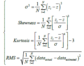
In this study, the porosity data from the Douala Basin were used to test and compare the results of three interpolation methods. A variographic analysis was conducted to see the difference between the interpolated data and the field data. This analysis enables to characterize the level of spatial correlation of the porosity data and to understand the behavior of the variograms. The geometric anisotropy of field data has been observed. The three interpolation methods proved their robustness by giving better statistical results for all the data. Each method showed its dependence on Variance, Skewness, Kurtosis, Standard deviation, and Root mean square.
We demonstrated that the interpolated data exhibited strong spatial correlations and were of better quality. These data allowed generating new interpolated variograms which had a better resolution, a better precision and a better coherence because the size of the angular window was reduced. The accuracy of these results has been evaluated. We found that the interpolation results are sensitive to the method.
The best mapping results of the porosity values were obtained with the kriging and the minimum curvature methods. On the other hand, in terms of statistical analysis, the three methods have had better precision results (Appendix).
Conflict of Interest
The authors declare that they have no competing interests.
Acknowledgements
This work was supported by the Department of Mines, Petroleum, Gas and Water Resources Exploration of the Faculty of Mines and Petroleum Industries of the University of Maroua, Cameroon. We thank the two referees who allowed a good consolidation of this paper
Appendix
The formulas of the statistical position and scattering parameters are presented in Tables 4 and 5.
| Gridding Methods | Variance | Skewness | Kurtosis | Standard deviation | Root mean square |
|---|---|---|---|---|---|
| Inverse distance to a power | 0.344066931153 | -0.582020710795 | 4.51218592545 | 0.586572187504 | 14.7293852714 |
| Minimum curvature | 1.29989698496 | 0.485239298528 | 4.7288324057 | 1.14013024912 | 14.8235152751 |
| Kriging | 0.699775803577 | -0.387452541244 | 3.28863158642 | 0.836526032815 | 14.7620141471 |
Table 4: Gridding and variogram report for univariate statistics.
| Gridding Methods | Variance | Skewness | Kurtosis | Standard deviation | Root mean square |
|---|---|---|---|---|---|
| Inverse distance to a power | 0.74496784134 | 0.140334227512 | 2.25701496992 | 0.863115195869 | 0.857965870441 |
| Minimum curvature | 0.246694544183 | 0.0121489328356 | 3.27114098627 | 0.496683545311 | 0.493946235602 |
| Kriging | 0.62893908605 | -0.179443087001 | 2.82586160136 | 0.793056798754 | 0.788595835729 |
Table 5: Cross validation report for univariate statistics (Cross validation provides root means squares error which measures the precision of each model fit to experimental yield variogram).
References
- Hatvani IG, Horváth J (2016) A Special Issue: Geomathematics in practice: Case studies from earth-and environmental sciences- Proceedings of the Croatian-Hungarian Geomathematical Congress, Hungary 2015. Open Geosciences 8: 1-4.
- Krige DG (1951) A statistical approach to some basic mine valuation problems on the Witwatersrand. J Southern African Institute of Mining and Metallurgy 52: 119-139.
- Matheron G (1963) Principles of geostatistics. Economic Geology 58: 1246-1266.
- Hohn ME (1999) Geostatistics and petroleum geology (2nd edn) Springer Science, Business Media Dordrecht, The Netherlands.
- Herzfeld UC (2004) Atlas of Antarctica: Topographic maps from geostatistical analysis of satellite radar altimeter data. Springer, Berlin.
- Monestiez P, Petrenko A, Leredde Y, Ongari B (2004) Geostatistical analysis of three dimensional current patterns in coastal oceanography: Application to the gulf of Lions (NW Mediterranean Sea). In: geoenv IV-Geostatistics for Environmental Applications, Barcelona, Spain, pp. 367-378.
- Kovács J, Korponai J, Kovács IS, Hatvani IG (2012) Introducing sampling frequency estimation using variograms in water research with the example of nutrient loads in the Kis-Balaton Water Protection System (W Hungary). Ecological Engineering 42: 237-243.
- Hatvani IG, Magyar N, Zessner M, Kovács J, Blaschke AP (2014) The Water framework directive: Can more information be extracted from groundwater data? A case study of Seewinkel, Burgenland, Eastern Austria. Hydrogeol J 22: 779-794.
- Kern Z, Kohán B, Leuenberger M (2014) Precipitation isoscape of high reliefs: interpolation scheme designed and tested for monthly resolved precipitation oxygen isotope records of an Alpine domain. Atmospheric Chemistry and Physics 14: 1897-1907.
- Deutsch JL, Palmer K, Deutsch CV, Szymanski J, Etsell TH (2016) Spatial modeling of geometallurgical properties: Techniques and a case study. Natural Resources Research 25: 161-181.
- Kohán B, Tyler J, Jones M, Kern Z (2017) Variogram analysis of stable oxygen isotope composition of daily precipitation over the British Isles. In: EGU General Assembly Conference Abstracts, Vienna, Austria 19: 12989-12990.
- Forti MJ (1999) Spatial statistics in landscape ecology. In: Landscape ecological analysis: Issues and applications, pp: 253-279.
- Webster R, Oliver MA (2001) Geostatistics for Environmental Scientists (2nd edn) John Wiley & Sons, Chichester.
- Kint V, Van Meirvenne M, Nachtergale L, Geudens G, Lust N (2003) Spatial methods for quantifying forest stand structure development: A comparison between nearest-neighbor indices and variogram analysis. Forest Science 49: 36-49.
- Zhao S, Zhou Y, Wang M, Xin, X, Chen F (2014) Thickness, porosity, and permeability prediction: comparative studies and application of the geostatistical modeling in an Oil feld. Environmental Systems Research 3: 1-24.
- Hatvani IG, Leuenberger M, Kohán B, Kern Z (2017) Geostatistical analysis and isoscape of ice core derived water stable isotope records in an Antarctic macro region. Polar Science 13: 23-32.
- Abdideh M, Bargahi D (2012) Designing a 3D model for the prediction of the top of formation in oil felds using geostatistical methods. Geocarto International 27: 569-579.
- Akin RO, Mullins D (2008) Capping protein increases the rate of actin-based motility by promoting filament nucleation by the Arp2/3 complex. Cell 133: 841-851.
- Esmaeilzadeh S, Afshari A, Motafakkerfard R (2013) Integrating artifcial neural networks technique and geostatistical approaches for 3D geological reservoir porosity modeling with an example from one of Iran’s oil fields. Petroleum Science and Technology 31: 1175-1187.
- Amanipoor H, Ghafoori M, Reza G, Lashkaripour (2013) The Application of geostatistical methods to prepare the 3D petrophysical model of oil reservoir. Open J Geol 3: 7-18 .
- Venegas JM, Herrera GS, Díaz-Viera MS, Manzanilla AV (2013) Geostatistical simulation of spatial va riability of convective storms in Mexico City Valley. Geofísica Internacional 52: 111-120
- Obi DA, Ilozobhie AJ, Abua JU (2015) Interpretation of aeromagnetic data over the Bida Basin, North Central, Nigeria. Advances in Applied Science Research 6: 50-63.
- Nguene FR, Tamfu S. Loule JP, Ngassa C (1992) Paleoevironments of the Douala and Kribi-Campo Sub-Basins in Cameroon, West Africa. In: Curnelle R (ed) Géologie Africaine. Bulletin du Centre de Recherche Exploration Production Elf-Aquitaine, Memoire13: 129-139.
- SNH (2005) Synthesis on the Rio Del Rey Basin and the Douala / Kribi-Campo Basin. Report interne.
- Golden Software (2002) Surfer 8 Users’ Guide, Golden Software Inc, Golden, Colorado.
- Cressie NAC (1993) Statistics for Spatial Data, John Wiley & Sons Press, New York, USA.
- Deutsch CV, Journel AG (1998) Geostatistical software library and user’s guide. Oxford University Press, New York.
- Arnaud M, Emery X (2000) Estimation and spatial interpolation: deterministic methods and geostatistical methods. HermLs science publications, Paris.
- Clark I, Harper WV (2000) Practical Geostatistics 2000. Ecosse North America lie. Columbus Ohio, USA.
- Srivastava II (1989) An introduction to applied geostatistics. Oxford University press. New York, USA.
- Wackernagel, Rees W (1998) Our ecological footprint: Reducing human impact on the earth. New society publishers, Canada.
- Ian CB (1974) Machine contouring using minimum curvature. Geophysics 39: 39-48.
- Burgess TM, Webster R (1980) Optimal interpolation and isarithmic mapping of soil properties. European J Soil Science 31: 315-331.
- Bastin G, Gevers M (1985) Identifcation and optimal estimation of random felds from scattered point-wise data. Automatica 21: 139-155.
- Cressie N (1988) Spatial prediction and ordinary kriging. Mathematical Geology 20: 405-421.
- Emery X (2009) The kriging update equations and their application to the selection of neighboring data. Computational Geosciences 13: 269-280.
- Costantino D, Angelini MG (2017) Production of DTM quality by TLS data. European J Remote Sens 46: 1-24.