Spanish
  Chinese
  Russian
  German
  French
  Japanese
  Portuguese
  Hindi
Hindi Research Article, Geoinfor Geostat An Overview Vol: 6 Issue: 2
Gravity Data Transformation by Polynomial Fitting and Kriging Data Analysis of the Mamfe Basin (Cameroon)
Nguimbous-Kouoh JJ1*, Ndougsa-Mbarga T2 and Manguelle-Dicoum E3
1Department of gas and petroleum exploration, Faculty of Mines and Petroleum Industries, University of Maroua, Cameroon
2Department of Physics, Advanced Teacher’s Training College, University of Yaounde, Yaounde, Cameroon
3Department of Physics, Faculty of Science, University of Yaounde, Yaounde, Cameroon
*Corresponding Author : Nguimbous-Kouoh JJ
Department of gas and petroleum exploration, Faculty of Mines and Petroleum Industries, University of Maroua, Cameroon
Tel: (+237) 696 383 408
E-mail: nguimbouskouoh@yahoo.fr
Received: April 06, 2018 Accepted: May 16, 2018 Published: May 23, 2018
Citation: Nguimbous-Kouoh JJ, Ndougsa-Mbarga T, Manguelle-Dicoum E (2018) Gravity Data Transformation by Polynomial Fitting and Kriging Data Analysis of the Mamfe Basin (Cameroon). Geoinfor Geostat: An Overview 6:2. doi: 10.4172/2327-4581.1000181
Abstract
Thirty-six gravity Bouguer data were collected in the Mamfe sedimentary basin. Third-order polynomial filtering was applied to the data. Third-order regional and residual gravity data were plotted as boxplots to compare distributions of different gravity fields. Boxplots enable to observe outliers in the data. These values
allowed for a more detailed study of the observed regional and residual anomaly values as they could have a significant impact on the results. Boxplots also found that the gravity data showed asymmetry. The kriging analysis procedure was initiated to describe the spatial variability of the different gravity data. The Gaussian
theoretical model was used to test anisotropy. The anisotropy test has shown that regional and residual gravity data exhibit geometric anisotropy and that spatial continuity is not necessarily the same in all directions. The unidirectional interpolated variograms were fitted with a tolerance of between 4° and 71° and a direction between -52° and 159°. 3D wireframe maps were created to map gravity fields in three-dimensional form and evaluate interpolated surfaces.
Keywords: Mamfe basin; Polynomial fitting; Boxplot analysis; Kriging analysis
Introduction
Geostatistics includes a number of methods and techniques for analyzing the spatial variability of spatially distributed or spatially structured variables [1]. The techniques developed by Krigeet al. [2] and Matheronet al. [3] to evaluate mineralized bodies have been disseminated in many fields using spatial data. These various disciplines include petroleum geology [4], hydrogeology Hatvan et al. [5], hydrology Kovács et al. [6], meteorology Kohán et al. [7], oceanography Monestiez et al. [8], geochemistry Kern et al. [9], metallurgy Deutsch et al. [10], geography Herzfeldet al. [11], Hatvani et al. [12], environmental control Kint et al. [13], landscapeecology Webster et al. [14], soil science, and agriculture Fortin et al. [15] and Zhao et al. [16]. In the petroleum industries, geostatistics is successfully applied to characterize oil reservoirs on the basis of interpretations from sparsely localized data such as reservoir thickness, porosity, permeability, seismic data, gravity field or magnetic field data [17-20]. One of the most used geostatistical techniques for interpolation of spatial data is the kriging technique. Kriging is a complex interpolation method and is considered as a method of estimating a regionalised variable at selected grid points. It can predict unbiased interpolation values with minimal variance [20,21].
In any kriging analysis, there are several main steps. These steps consist of creating an experimental semi-variogram, linking a theoretical model to the experimental semi-variogram and using the latter’s information to perform kriging. More generally, this may be Determine appropriate theoretical models of semi-variogram; check the possibility of anisotropy of the experimental semi-variogram; generate kriging estimates and estimation errors, i.e., Kriging errors, for a point, area or volume; mapping the spatial distributions of kriging estimates and kriging errors. In a kriging analysis, all these components must be systematically taken into account [22-27] . What we can notice is that the analysis of spatial continuity or roughness of geospatial data in different directions and tolerances takes time [28-31].
The aims of this study are: to carry out the polynomial filtering of the Bouguer data of the mamfe basin, to plot the boxplots to understand the influence of the outliers in the data and to compare the distributions of the Bouguer gravity fields, regional and residual then to realize a kriging analysis of gravity data of the basin and their cartographies.
Location of the Study Area
The Mamfe sedimentary basin (Figure 1) is an intracratonique rift basin formed in response to the dislocation of the Gondwana supercontinent and following the separation of South American and African plates. The basin is a small extension of the Benue sedimentary basin. The basin is favorable to the exploration and exploitation of salt springs, minerals, precious stones and hydrocarbons. It has an area of approximately 2400 km2 and is located between latitudes 5°30’N and 6°00’N and longitudes 8°40’ E and 9°50’E (Figure 1). It has the form of a plain with an average altitude that varies between 90 and 300 m above the sea level.

Figure 1: Geological map of the Mamfe sedimentary basin [40].
Figure 1 shows the available geological map of the basin. Some geological details were extrapolated or removed. The geological map is preliminary and has jointly been updated following several studies [32-41]. The geomorphology of the area is characterized by a succession of horst and grabens. Overall, the Mamfe sedimentary basin has a NW-SE structural trend with a length of 130 Km and a width of approximately 60 km. It is bordered by faults, lineaments and rivers such as Manyu, Munaya and extends from Cameroon to Nigeria [32-41].
Data Acquisition and Processing
Figure 2 shows the distribution of gravity data collected through the Mamfe Basin. It is deduced from the Cameroon gravity database that manages the RID (Research Institute for Development). The Lacoste-Romberg gravimeter (1975-1976) was used for data recording. The determination of the altitudes was made by barometric leveling with a Wallace-Tiernan altimeter. The RID gravity network established in Douala served as a reference base for measurements. The spatial reference coordinate system used is WGS84 and the data projection system is UTM.

Figure 2: Map of collecting data of the Mamfe sedimentary basin.
The Bouguer anomaly was calculated at each station using the expression by Poudjom et al. [42]: B=G-(Go-Cz-T) Where G is the observed value of the gravitational field and its expression is: G=Gr+ΔG with Gr the value of the gravity field in a adopted station as reference and ΔG measuring the gravity field difference between the reference station and a given station. Go is the theoretical value of the gravitational field at the point of the reference ellipsoid corresponding to the station. Go has been defined in the IGSN71 reference system whose formula is:
Go=978031.8 (1+0.053024sin Õ2)-0.0000022sin2Õ2
The error on the latitude of a station is considered between 0.2 mgal and 0.5 mgal with Õ=3°.
• Cz: is the Bouguer correction
• It represents the sum of the correction of the free air C1(mgal)=0.3086 Z and the plateau correction C2(mgal)=- 0.0419dZ Where d is the density of the crust and Z the altitude of the station expressed in meters. For the reasons of homogeneity we adopted d = 2.67 for all the stations from where Cz(mgal)=0.1967Z. The imprecision of the barometric leveling has led to an error on Cz generally less than 1 mgal but which has reached 2 or 3 mgal in unfavorable cases.
• T: relief correction. It takes into account the relief around the station. The anomaly value at each point was tainted with a maximum error of 5 mgal in the worst conditions, in most cases the error remained below 3 mgal.
Materials and Methods
In linear geostatistics the choice of software and an interpolation method are very important for spatially analyzing a variable of interest [1-4]. We used R software Ihaka et al. [43] and Surfer Golden Software [44]. Surfer is a 2D and 3D surface mapping program that transforms random data into contours of continuous curved faces. Surfer uses twelve different methods to interpolate data; R is statistical software created by Ihaka et al. [43]. It is both a computer language and a work environment: the commands are executed by means of instructions coded in a relatively simple language, the results are displayed in text form and the graphics are displayed directly in a window of their own. This software is used for manipulating data, graphing and statistical analysis of this data.
In this part, we expose the polynomial fitting method and the different steps of the kriging method in the univaried framework.
The polynomial separation method
The polynomial separation method was used to produce the third degree regional and residual maps. The algorithm by Gupta and Murthy et al. [45,46] was used to adjust the polynomial surfaces to the Bouguer anomaly map. This method is based on the analytical least square method and the polynomial decomposition series.
The least-square method is used to compute the mathematical surface which gave the best fits to the gravity field within specific limits [45-47]. This surface is considered to be the regional gravity anomaly. The residual is obtained by subtracting the regional field from the observed gravity field. In practice, the regional surface is considered as a two-dimensional polynomial. The order of this polynomial depends on the complexity of the geology in the study area. The third-order polynomial surfaces of the regional anomaly obtained in this work is presented and the corresponding residual anomaly.
Mathematic formulation of the method
The Bouguer anomaly B(x, y) in the given point M(x, y) of the earth in Cartesian coordinates is governed by the relation:
B(xi, yi)= A(xi, yi)+ R(xi, yi) (1)
B(xi, yi) is the sum of the residual anomaly A(xi, yi) and the regional anomaly R(xi, yi).
The surface F(xi, yi) which is adapted to the gravity field data g(x,y) is given by the following relation [45-49]:
 (2)
(2)
Where N is the order of the polynomial,  the number of terms of the polynomial, and CM the coefficients to be determined:
The first order Polynomial is:
F(xi,yi)=C1+C2Xi+C3Yi (3)
The second order polynomial is:
 (4)
(4)
The third order polynomial is:
 (5)
(5)
We denote byεi= B(xi, yi)- F(xi, yi) the difference between the homologous points of the experimental and analytical surfaces respectively and by N0 the number of stations Pi in which the Bouguer anomaly is known. The adjustment of the surfaces which consists in making the quadratic deviation minimal is expressed by:
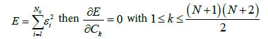 (6)
(6)
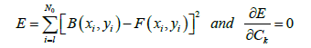
We then obtain a system of (M) equations with (M) unknowns. The unknowns are the coefficients Ck of the polynomial F(xi, yi) of order N. Once the coefficients are determined we determine the analytic regional anomaly R(xi, yi) =F(xi, yi) and the residual by:
A(xi, yi)= B(xi, yi)- F(xi, yi) (7)
The polynomial method is particularly used when the amplitude of the residual anomalies is negligible compared to the regional one. Apart from the polynomial method there are other methods such as the upward continuation method.
Variographic formalism and kriging
In a classical framework, kriging analysis generally involves two stages: the variogram estimation and the use of the model coefficients for Kriging [17-20].
The formalism of variographic estimation: The variogram is the basic tool in kriging analysis and is required for geostatistical spatial prediction. The variogram is estimated by the experimental variogram γ*(h), which is calculated from the discrete data as follows [17-20]:
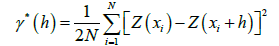
where N is the number of pairs of points distant from h.
Once the experimental variogram has been calculated, it is necessary to replace it with a theoretical variogram whose coefficients are estimated by a least squares procedure [20].
There are several types of theoretical variogram models used for kriging [17-20]:
The spherical variogram is characterized by :
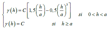
With a the range, h the interpolation step and C the constant sill
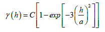
The Gaussian variogram is characterized by:
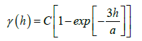
The exponential variogram is characterized by:
The power variogram is characterized by:
For b = 1,the variogram is linear; b = 2,the variogram is a parabola
The formalism of variographic anisotropy: There are different types of anisotropies which enable to know the different orientations that spatialized data can take [17-20]. Geometric anisotropy is the simplest case. A geometric anisotropy is reflected in the experimental variograms by a range which varies according to the direction. Geometric anisotropy is observed when the variogram respects the following mathematical formulation:
With ag the maximum range, ap the minimum range and aθ the range in the anisotropy direction θ
Anisotropy is called zonal when it cannot be solved by a simple geometric or linear coordinate’s transformation. It causes for the bearing variogram which varies according to the space direction.
The kriging formalism
Kriging is an interpolation method that gives the best unbiased linear estimate of the point value of a regionalised variable [2,3]. The kriging interest is that it enable to calculate the estimation error i.e the kriging variance [2,3]. It allows the taking into account of: the data configuration; the distance between data and targets; spatial correlations and external information. Kriging is an exact interpolator, it has a screen effect, it is almost without conditional bias. It is transitive, generally performs a smoothing and takes into account the field size to estimate and the position of the points between them [2,3].
The mathematic formulation of kriging imposes the minimization of the following variance [1-4]:

Where Zv represents the known values at different points and:
 is the estimator
λi is the weight and Zi is the random variable corresponding to each point.
Since kriging is an unbiased interpolator then:

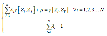
To minimize the kriging variance we use the Lagrangian [1-4]:
With μ the Lagrange multiplier
By calculating:  and
and  we obtain the system of equation:
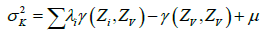
The variance of kriging is given by:
In order to solve the system numerically, it is convenient to write it in matrix form AX=B We obtain:
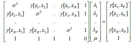
The system allows finding the set of weights λi and the Lagrange multiplier μ that minimize the variance and make the estimator unbiased. The variance of kriging is then obtained by the following formula:
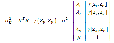
With the XT transpose of X=A-1B
The system of equations can also be expressed in terms of covariance under the assumption that the random process is stationary.
Results
In this part, we present the results of polynomial separation by boxplots, variographic analysis and data mapping.
Polynomial separation boxplots analysis
It is interesting to use box-plots when you want to visualize concepts such as the symmetry, the dispersion or the centrality of the values distribution associated with a variable. They are also very interesting for comparing variables based on similar scales. The graphs (Figure 3) represent Bouguer’s gravity fields and interpolated regional and residual data. They show different shapes and positions of box-plots. These graphs enable to summarize the gravity data in a simple and visual way, to identify the extreme values and to understand the different anomaly values distribution.

Figure 3: Box-plots representing Bouguer anomalies, regional and residual: a) field data and b) interpolated data.
It can be noted that overall 50% of gravity anomaly values are inside each box. The values outside the box plots are represented by dots. It cannot be considered that if an observed value is outside the box-plots then it is an outlier. However, this indicates that this observed value needs to be studied in more detail. Outliers are data values that are far removed from other data values and can have a significant impact on the results.
These boxes have variable widths, it is not a simple aesthetic transformation, and the width is proportional to the size of the anomaly values. The widths of the two parts of the box-plot reflect the dispersion of the values located at the center of the series (the box contains 50% (approximately) of all anomalies: 25% at the top of the median and 25% at the bottom); in general, the boxplots will be all the more extensive as the dispersion of the series of values is great.
The median is represented by the line in the box. The median is a common measure of data centering. Half of the values are lower or equal and half of the values are greater or equal.
When the data is asymmetrical, the majority of them are located on the upper or lower side of the graph. Asymmetry indicates that the data may not be normally distributed (Table 1).
| Number | X (Longitudes) | Y (Latitudes) | Bouguer anomalies | Regional anomalies | Residual anomalies |
|---|---|---|---|---|---|
| 1 | 9,636 | 5,691 | -44 | -4,7204 | 6,72024 |
| 2 | 9,592 | 5,687 | -43 | 2,75236 | 1,24764 |
| 3 | 9,567 | 5,679 | -42 | 3,18388 | -1,18388 |
| 4 | 9,487 | 5,701 | -39 | 3,51149 | -3,51149 |
| 5 | 9,463 | 5,697 | -36 | 3,25523 | -5,25523 |
| 6 | 9,439 | 5,696 | -32 | 3,31059 | -5,31059 |
| 7 | 9,352 | 5,701 | -20 | -0,17256 | -2,82744 |
| 8 | 9,313 | 5,727 | -18 | 0,14928 | -4,14927 |
| 9 | 9,3 | 5,716 | -15 | 0,53131 | -3,53131 |
| 10 | 9,304 | 5,739 | -16 | -1,55684 | 0,55684 |
| 11 | 9,294 | 5,694 | -12 | -5,82415 | 9,82415 |
| 12 | 9,415 | 5,671 | -28 | -6,51968 | 3,51968 |
| 13 | 9,436 | 5,641 | -30 | -10,72953 | 7,72953 |
| 14 | 9,451 | 5,617 | -31 | -10,98765 | 5,57853 |
| 15 | 9,456 | 5,598 | -33 | -12,57853 | 4,98765 |
| 16 | 9,483 | 5,592 | -36 | -13,15335 | 6,15335 |
| 17 | 9,5 | 5,571 | -33 | -13,37963 | 5,37963 |
| 18 | 9,517 | 5,562 | -27 | -13,15335 | 1,65255 |
| 19 | 9,263 | 5,685 | -8 | -11,47765 | -3,52235 |
| 20 | 9,234 | 5,678 | -7 | -9,4475 | -6,5525 |
| 21 | 9,201 | 5,674 | -7 | -11,03323 | -6,96677 |
| 22 | 9,184 | 5,682 | -6 | -15,87953 | -4,12047 |
| 23 | 9,159 | 5,679 | -3 | -23,30415 | -4,69585 |
| 24 | 9,126 | 5,706 | -3 | -28,72188 | -1,27812 |
| 25 | 9,062 | 5,742 | -1 | -33,31109 | 2,31109 |
| 26 | 9,023 | 5,761 | -3 | -36,71332 | 3,71332 |
| 27 | 8,997 | 5,756 | -4 | -39,55585 | 3,55585 |
| 28 | 8,974 | 5,753 | -3 | -44,39541 | 11,39541 |
| 29 | 8,949 | 5,784 | -3 | -47,23789 | 20,23789 |
| 30 | 8,938 | 5,799 | -2 | -22,00851 | -9,99138 |
| 31 | 8,857 | 5,812 | 4 | -23,66246 | -1,27812 |
| 32 | 8,89 | 5,808 | 2 | -25,08232 | -13,91768 |
| 33 | 8,921 | 5,806 | 0 | -34,16419 | -7,83581 |
| 34 | 9,101 | 5,708 | 4 | -35,62284 | -7,37716 |
| 35 | 8,8 | 6,03 | 2 | -39,54111 | -4,45889 |
| 36 | 9,66 | 6,03 | -35 | -49,29324 | 14,29324 |
Table 1: Bouguer anomaly values as well as regional and residual anomalies obtained from polynomial separation.
Variographic analysis of the data
Variographic analysis plays a key role in the process of assessing the correlation level of spatialized data and their modeling. It indicates problems related to data dispersion and allows kriging or mapping in a particular area [17-20].
Anisotropy analysis of the field data
Figure 4 shows the variograms of all Bouguer gravity data, regional and residual. Each variogram is represented by the cloud, the experimental variogram and the three theoretical models selected for the anisotropy tests. The experimental variogram is a graph that shows the contributions of each pair of points to the final variogram. The scatter plot gives a visual impression of the dispersion of values at different offsets. He has no precise direction. We chose a direction and a tolerance each time to obtain an unidirectional variogram which enable to neglect the lag h.

Figure 4: Simulation of the gravity data anisotropy.
Anisotropy is the parameter that allows us to better know the spatial continuity of the values of Bouguer, regional and residual gravity fields. Figure 4 shows the simulation of theoretical Gaussian variograms across the experimental variograms cloud. These figures prove that bouguer, regional and residual gravity data present a geometric anisotropy. Spatial continuity is not necessarily the same in all directions. The Gaussian model fit the dataset quite well (Table 2).
| Bouguer Anomaly Data | ||
|---|---|---|
| Models | Anisotropy angle | Anisotropy ratio |
| Gaussien 1 (vert) | 105 | 2 |
| Gaussien 2 (jaune) | 115 | 1.8 |
| Gaussien 3 (bleu) | 140 | 2 |
| Regional Anomaly Data | ||
| Gaussien 1 (vert) | 140 | 1.54 |
| Gaussien 2 (jaune) | 100 | 1.4 |
| Gaussien 3 (bleu) | 10 | 0.7 |
| Residual Anomaly Data | ||
| Gaussien 1 (vert) | 30 | 3.3 |
| Gaussien 2 (jaune) | 45 | 0.2 |
| Gaussien 3 (bleu) | 15 | 0.1 |
Table 2: Characteristics of different models of anisotropy.
Variographic analysis of grid data
A variogram expresses the semi-variance of a regionalized variable and its variation as a function of the lag distance h. This variogram shows that, beyond a certain limit called range, no spatial correlation exists between the points. A theoretical variogram model is first computed to fit the experimental variogram obtained with the data, and is then used from Kriging [17-20].
The gridded data variograms are shown in Figure 5. The different experimental variograms clouds were fitted by the Gaussian theoretical variogram. The tolerances and directions chosen were a compromise between the need to have a sufficient number of pairs of points for calculating the variogram and the risk of too much smoothing of the curve. Overall the three variograms are unidirectional. The tolerance direction varies between 4° and 71° and the direction between -52° and 159°. These values were each time set so that the direction of any particular lag distance h, becomes unimportant (Table 3).
| Experimental variogram and Models | Max lag distance | Lag with | Vertical scale | Anisotropy ratio | Anisotropy Angle | Tolerance | Direction |
|---|---|---|---|---|---|---|---|
| Bouguer variogram | 71 | 0.1775 | 231.3 | 2.3 | 100 | 4 | 16 |
| Regional variogram | 0.32 | 0.0008 | 194.2 | 2 | 70 | 4 | 159 |
| Residual variogram | 0.32 | 0.0008 | 37.9 | 2 | 162.8 | 71 | -52 |
Table 3: Characteristics of fitted experimental variogram.

Figure 5: Fitted Variograms of gridded data (Experimental (line with markers) and theoretical semi-variogram (continuous line).
Interpretation of 3D wireframe maps
3D Wireframe map models are three-dimensional cartographic forms of the superficial and deep geological formations commonly used in geology and mining. The wireframe model maps a set of points with known triaxial Cartesian (x, y, z) coordinates. Before the plot, a grid routine is used to place the randomly located field data into a regular grid with selected spacing. The wireframe plot results in an open grid (x, y) with the anomaly of each grid node corresponding to the z coordinate at that point. The wireframe structures that we present in this part are three-dimensional representations of the gravity data of the Mamfe basin. These wireframe structures cannot be larger or smaller than the extent of the grid data file.
Bouguer 3D wireframemap
The Bouguer 3D wireframe map gives an idea of the structural distribution of the superficial and deep geological formations (Figure 6). It reflects the regular and continuous variations of the Bouguer gravity field of the Mamfe basin. The Bouguer 3D wireframe map indicates areas of existence of slopes and density discontinuities such as faults.

Figure 6: Bouguer 3D wireframe model with draped contours of the mamfe basin.
Regional 3D wireframe map
The Regional 3D wireframe map shows the overall gravity regional trends affecting the basement of the Mamfe Basin (Figure 7). These trends are N-S, E-W. This graph shows areas where the basement seems to have undergone a dilation confirming the hypothesis of magmatic upwelling in the basin; while the platform zone can be associated with a consolidation of the basement.

Figure 7: Regional 3D wireframe model with draped contours of the mamfe basin.
Residual 3D wireframemap
The Residual 3D wireframe map gives a three-dimensional representation of the sedimentary layer in the Mamfe basin (Figure 8). It is characterized by two negative gravity anomalies that can be associated with sedimentary infilling zones.

Figure 8: Residual 3D wireframe model with draped contours of the mamfe basin.
Conclusion
In this study, thirty six gravity Bouguer data were collected in the Mamfe sedimentary basin. Third-order polynomial filtering was applied to the data. Third-order regional and residual gravity data were obtained. The dataset was plotted as boxplots to understand the influence of the outliers in the data and then to compare Bouguer gravity field distributions, regional and residual. The kriging analysis procedure was initiated to: describe the spatial variability of the different gravity data; identify spatial correlations and different trends and directions of experimental semi-variograms; check the possibility of the experimental semi-variograms anisotropy ; fit interpolated semi-variogram models using mathematical functions; Create the 3D wireframe maps of the different gravity fields from the new data grids to evaluate the interpolated surfaces.
Acknowledgment
This study was conducted as part of the research activities conducted in the Department of Mines, Petroleum, Gas and Water Resources Exploration. Thank to all the colleagues involved in the application of geostatistics in the oil and mining field.
References
- Hatvani IG, Horváth J (2016) A Special Issue: Geomathematics in practice: Case studies from earth-and environmental sciences-Proceedings of the Croatian-Hungarian Geomathematical Congress, Hungary 2015. Open Geosciences 8: 1-4.
- Krige DG (1951) A statistical approach to some basic mine valuation problems on the Witwatersrand. Journal of the Southern African Institute of Mining and Metallurgy 52: 119-139.
- Matheron G (1963) Principles of geostatistics. Economic geology 58: 1246-1266.
- Hohn ME (1999) Geostatistics and Petroleum Geology. Springer Science & Business Media Dordrecht, The Netherlands.
- Hatvani IG, Magyar N, Zessner M, Kovacs J, Blaschke AP (2014) The Water Framework Directive: Can more information be extracted from groundwater data? A case study of Seewinkel, Burgenland, eastern Austria. Hydrogeology Journal 22: 779-794.
- Kovacs J, Korponai J, Kovacs IS, Hatvani IG (2012) Introducing sampling frequency estimation using variograms in water research with the example of nutrient loads in the Kis-Balaton Water Protection System (W Hungary). Ecological engineering 42: 237-243.
- Kohan B, Tyler J, Jones M, Kern Z (2017) Variogram analysis of stable oxygen isotope composition of daily precipitation over the British Isles. XIVth Workshop of the European Society for Isotope Research, Băile Govora, Romania.
- Monestiez P, Petrenko A, Leredde Y, Ongari B (2004) Geostatistical analysis of three dimensional current patterns in coastal oceanography: application to the gulf of Lions (NW Mediterranean Sea). GeoENV IV-Geostatistics for Environmental Applications 13: 367-378.
- Kern Z, Kohan B, Leuenberger M (2014) Precipitation isoscape of high reliefs: interpolation scheme designed and tested for monthly resolved precipitation oxygen isotope records of an Alpine domain. Atmospheric chemistry and physics 14: 1897-1907.
- Deutsch JL, Palmer K, Deutsch CV, Szymanski J, Etsell TH (2016) Spatial modeling of geometallurgical properties: techniques and a case study. Natural Resources Research 25: 161-181.
- Herzfeld UC (2012) Atlas of Antarctica: topographic maps from geostatistical analysis of satellite radar altimeter data. Springer Science & Business Media Dordrecht, The Netherlands.
- Hatvani IG, Leuenberger M, Kohan B, Kern Z (2017) Geostatistical analysis and isoscape of ice core derived water stable isotope records in an Antarctic macro region. Polar Science 13: 23-32.
- Kint V, Meirvenne VM, Nachtergale L, Geudens G, Lust N (2003) Spatial methods for quantifying forest stand structure development: a comparison between nearest-neighbor indices and variogram analysis. Forest science 49: 36-49.
- Webster R, Oliver MA (2007) Geostatistics for environmental scientists. John Wiley & Sons, USA.
- Fortin MJ (1999) Spatial statistics in landscape ecology. InLandscape ecological analysis. Springer, New York, USA.
- Zhao S, Zhou Y, Wang M, Xin X, Chen F (2014) Thickness, porosity, and permeability prediction: comparative studies and application of the geostatistical modeling in an Oil field. Environmental Systems Research 3: 7.
- Akin O, Mullins RD (2008) Capping protein increases the rate of actin-based motility by promoting filament nucleation by the Arp2/3 complex. Cell 133: 841-851.
- Abdideh M, Bargahi D (2012) Designing a 3D model for the prediction of the top of formation in oil fields using geostatistical methods. Geocarto International 27: 569-579.
- Esmaeilzadeh S, Afshari A, Motafakkerfard R (2013) Integrating Artificial Neural Networks Technique and Geostatistical Approaches for 3D Geological Reservoir Porosity Modeling with an Example from One of Iran's Oil Fields. Petroleum Science and Technology 31: 1175-1187.
- Amanipoor H, Ghafoori M, Lashkaripour GR (2013) The application of géostatistical methods to prepare the 3D petrophysical model of oil reservoir. Open Journal of Geology 3.
- Mendez-Venegas J, Herrera GS, Diaz-Viera MA, Valdes-Manzanilla A (2013) Geostatistical simulation of spatial variability of convective storms in Mexico City Valley. Geofísica Internacional 52: 111-120.
- Cressie NAC (1993) Statistics for Spatial Data, John Wiley & Sons Press, New York, USA
- Deutsch CV, Journel AG (1998) Geostatistical software library and user’s guide. Oxford University Press, New York, USA.
- Clark I, Harper WV (2000) Practical Geostatistics 2000. Ecosse North America lie, Columbus, Ohio, USA.
- Isaaks EH, Srivastava RM (1989) An introduction to applied geostatistics. Oxford University press, New York, USA.
- Wackernagel M, Rees W (1998) Our ecological footprint: reducing human impact on the earth. New Society Publishers, USA.
- Arnaud M, Emery X (1999) Estimation et interpolation de donnees spatiales. CIRAD, Montpellier, France.
- Burgess TM, Webster R (1980) Optimal interpolation and isarithmic mapping of soil properties I The Semi-Variogram and Punctual Kriging. Europ J Soil Sci : 315-331.
- Bastin G, Gevers M (1985) Identification and optimal estimation of random fields from scattered point-wise data. Automatica 21: 139-155.
- Cressie N (1988) Spatial prediction and ordinary kriging. Mathematical geology 20: 405-421.
- Emery X (2009) The kriging update equations and their application to the selection of neighboring data. Computational Geosciences 13: 269-280.
- Eseme E, Littke R, Agyingi CM (2006) Geochemical characterization of a Cretaceous black shale from the Mamfe Basin, Cameroon. Petroleum Geoscience 12: 69-74.
- Eseme E, Abanda PA, Agyingi CM, Foba-Tendo J, Hannigan RE (2006) Composition and applied sedimentology of salt from brines of the Mamfe Basin, Cameroon. Journal of Geochemical Exploration 91: 41-55.
- Nguimbous-Kouoh JJ (2003) Structural Interpretation of the Mamfe Sedimentary Basin of Southwestern Cameroon along the Manyu River Using Audiomagnetotellurics Survey. ISRN Geophysics 20: 52-59.
- Nouayou R (2005) The use of Aeromagnetic Data Interpretation to Characterize the Features in the Mamfe Sedimentary Basin Cameroon and a Part of the East of Nigeria. International Journal of Science and Research 6: 617-624.
- Tabod CT, Kamga AT, Dicoum EM, Nouayou R, Nguiya S (2006) An Audio-Magnetotelluric Investigation of The Eastern Margin of The Mamfe Basin, Cameroon. The Abdus Salam International Centre for Theoretical Physic, Trieste, Italy.
- Ndougsa-Mbarga T, Manguelle-Dicoum E, Campos-Enriquez JO, Yene Atangana Q (2007) Gravity anomalies, sub-surface structure and oil and gas migration in the Mamfe, Cameroon-Nigeria, sedimentary basin. Geofísica internacional 46: 129-139.
- Ajonina HN, Betzler C, Jaramillo C (2010) Paleoclimatic significance of an Early Cretaceous fan-delta sedimentary succession in the Eastern Mamfe Basin, SW Cameroon. In the proceedings of Afrikagruppe deutscher Geowissenschaftler (AdG), Frankfurt, Germany.
- Ajonina HN, Jaramillo C, Volkheimer W, Mejía P, Betzler C, et al. (2010) Palynostratigraphy and age of the Lower Cretaceous Mamfe Group, Mamfe Basin, SW Cameroon, eastern West Africa. In the proceedings of 8th European Palaeobotany-Palynology Conference, Budapest, Hungary.
- Ajonina HN, Betzler C, Hell JV, Eseme E, Volkheimer W, et al. (2012) Hydrocarbon potential of the Mamfe Basin, SW Cameroon. GV & Sediment Meeting 2012, Hamburg, Germany.
- Eyong JT, Wignall P, Fantong WY, Best J, Hell JV (2013) Paragenetic sequences of carbonate and sulphide minerals of the Mamfe Basin (Cameroon): Indicators of palaeo-fluids, palaeo-oxygen levels and diagenetic zones. Journal of African Earth Sciences 86: 25-44.
- Poudjom-Djomani YH, Boukeke DB, Legeley-Padovani A, Nnange JM, Ateba B, et al. (1996) Levés gravimétriques de reconnaissance-Cameroun. Orstom, Paris.
- Ihaka R, Gentleman R (1996) R: a language for data analysis and graphics. Journal of computational and graphical statistics 5: 299-314.
- Golden Software (2002) Surfer 8. Users’ Guide Golden Software Inc, Colorado, USA.
- Gupta VK (1983) A Least Squares Approach to Depth Determination from Gravity Data. Geophysics 48: 357-360.
- Murthy IVR, Krisshnamacharyulu SKG (1990) A Fortran 77 Programme to Fit a Polynomial of Any Order to Potential Field Anomalies. Journal of Association of Exploration Geophysicists 11: 99-105.
- Nguimbous-Kouoh JJ, Ngos III S, Mbarga TN, Manguelle-Dicoum E (2017) Use of the Polynomial Separation and the Gravity Spectral Analysis to Estimate the Depth of the Northern Logone Birni Sedimentary Basin (CAMEROON). International Journal of Geosciences 8: 14-42.
- Eseme E, Agyingi CM, Foba-Tendo J (2002) Geochemistry and genesis of brine emanations from Cretaceous strata of the Mamfe Basin, Cameroon. Journal of African Earth Sciences 35: 467-476.
- Nguimbous-Kouoh JJ (2010) The structure of the Goulfey-Tourba sedimentary basin (Chad-Cameroon): A gravity study. Geofísica Internacional 49: 181-193.